Scale-Invariant Feature Transform (SIFT) is an old algorithm presented in 2004, D.Lowe, University of British Columbia. However, it is one of the most famous algorithm when it comes to distinctive image features and scale-invariant keypoints.
Summary
- Problem Statement
- Proposed methods before SIFT (e.g. Harris corner) are not invariant to image scale and rotation.
- Research Objective
- To find a method for extracting distinctive invariant features from images that can be used to perform reliable matching between different views of an object or scene.
- Proposed Solution
- Scale-space extrema detection
- Keypoint localization
- Orientation assignment
- Keypoint descriptor
- Contribution
- The features are invariant to image scale and rotation, and are shown to provide robust matching across a substantial range of affine distortion, change in 3D viewpoint, addition of noise, and change in illumination.
- The features are highly distinctive, in the sense that a single feature can be correctly matched with high probability against a large database of features from many images.
- The authors described an approach to using these features for object recognition.
- It could robustly identify objects among clutter and occlusion while achieving near real-time performance.
Proposed Method
There are four major stages of computation to generate the set of image reatures.
1. Scale-space extrema detection
First stage searches over all scales and image locations. It is implemented efficiently by using a difference-of-Gaussian function to identify potential interest points that are invariant to scale and orientation.
- Firstly, Laplacian of Gaussian (LoG) was used to detects blobs in various sizes.
- As LoG is costly, SIFT algorithm uses Difference of Gaussians (Dog) which is an approximation of LoG.
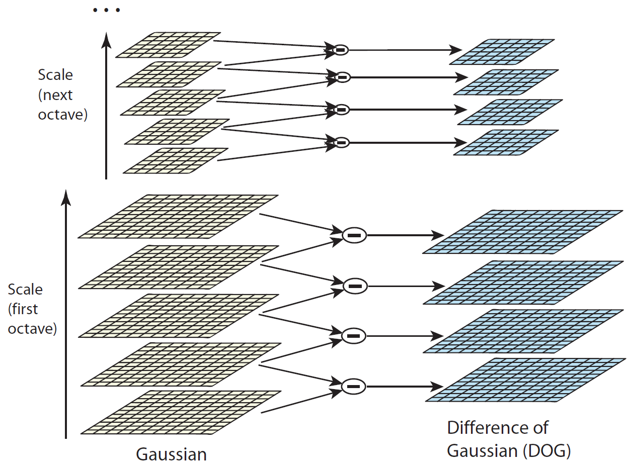 Figure 1: For each octave of scale space, the initial image is repeatedly convolved with Gaussians to produce the set of scale spaces shown on the left. Adjacent Gaussian images are subtracted to produce the difference-of-Gaussian images on the right. After each octave, the Gaussian image is down-sampled by a factor of 2, and the process repeated.
- Once DoG are found, images are searched for local extrema over scale and space.
- If it is a local extrema, it is a potential keypoint.
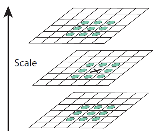 Figure 2: Maxima and minima of the difference-of-Gaussian images are detected by comparing a pixel (marked with X) to its 26 neighbors in 3x3 regions at the current and adjacent scales (marked with circles).
2. Keypoint localization
At each candidate location, a detailed model is fit to determine location and scale. Keypoints are selected based on measures of their stability.
- Once potential keypoints locations are found, it has to be refined to get more accurate results.
- SIFT use Taylor series expansion of scale space to get more accurate location of extrema
- If the intensity at this extrema is less than a threshold value, it is rejected.
- DoG has higher response for edges, so edges also need to be removed.
- For this, a concept similar to Harris corner detector is used.
- So it eliminates any low-contrast keypoints and edge keypoints and what remains is strong interest points.
3. Orientation assignment
One or more orientations are assigned to each keypoint location based on local image gradient directions. All future operations are performed on image data that has been transformed relative to the assigned orientation, scale, and location for each feature, thereby providing invariance to these transformations.
- A neighbourhood is taken around the keypoint location depending on the scale, and the gradient magnitude and direction is calculated in that region.
- An orientation histogram with 36 bins covering 360 degrees is created.
- The highest peak in the histogram is taken and any peak above 80% of it is also considered to calculate the orientation.
- It creates keypoints with same location and scale, but different directions, and it contribute to stability of matching.
4. Keypoint descriptor
The local image gradients are measured at the selected scale in the region around each keypoint. These are transformed into a representation that allows for significant levels of local shape distortion and change in illumination.
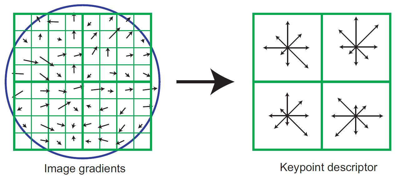 Figure 3: A keypoint descriptor is created by first computing the gradient magnitude and orientation at each image sample point in a region around the keypoint location, as shown on the left. These are weighted by a Gaussian window, indicated by the overlaid circle. These samples are then accumulated into orientation histograms summarizing the contents over 4x4 subregions, as shown on the right, with the length of each arrow corresponding to the sum of the gradient magnitudes near that direction within the region.
Keypoint Matching
Keypoints between two images are matched by identifying their nearest neighbours.
- If the second closest-match may be very near to the first, ratio of closest-distance to second-closest distance is taken and if it is greater than 0.8, they are rejected.
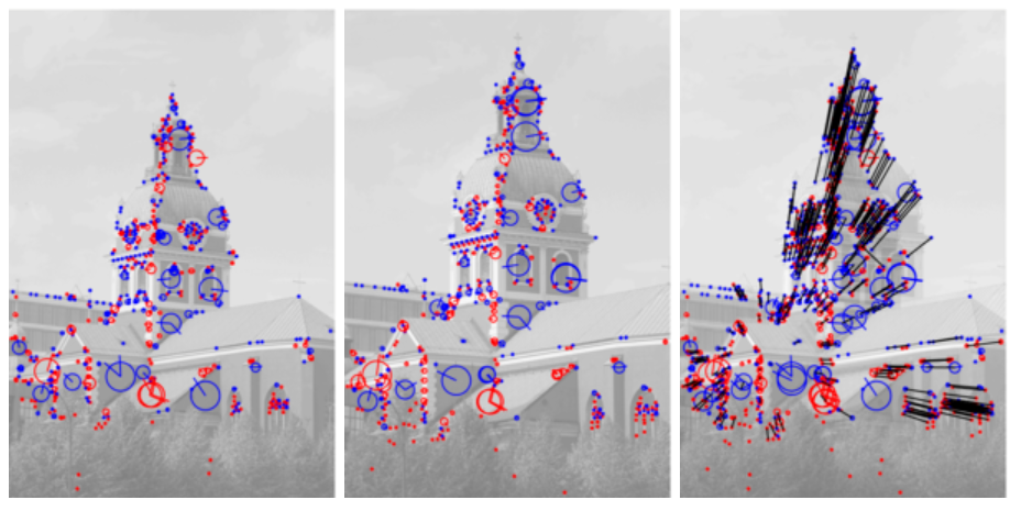 Figure 4: Interest points detected from two images of the same scene with the computed image matches drawn as black lines between corresponding interest points. The blu and red arrows at the centers of the circles illustrate the orientation estimates obtained from peaks in local orientation histograms around the interest points.
References
- Paper: Distinctive image features from scale-invariant keypoints, International Journal of COmputer Vision 2004
- It gives the most complete and up-to-date reference for the SIFT feature detector
- Paper: Object recognition from local scale-invariant features, ICCV 1999
- It gives the SIFT approach to invariant keypoint detection and some more information on the applications to object recognition
- Paper: Local feature view clustering for 3D object recognition
- It gives methods for performing 3D object recogniiton by interpolating between 2D views and a probabilistic model for verification of recognition
- Wikipedia
- OpenCV: Introduction to SIFT (Scale-Invariant Feature Transform)