It is always important what kind of optimization algorithm to use for training a deep learning model. According to the optimization algorithm we use, the model can produce better and faster results.
Optimization Algorithm
Optimization algorithm minimize or maximize an error function (objective function or loss function) for updating model’s internal learnable parameters \(W\) and \(b\).
Types of Optimization
Optimization Algorithm have 2 major categories:
-
First Order Optimization Algorithms: These algorithms minimize or maximize a Loss function \(E(x)\) using gradient values with respect to the parameters such as Gradient descent. The first order derivative tells us whether the function is decreasing or increasing at a particular point. First order Derivative basically give us a line which is Tangential to a point on its Error Surface.
-
Second Order Optimization Algorithms: It uses the second order derivative which is called Hessian to minimize or maximize the loss function. The Hessian is a Matrix of second order partial derivative. Since the second derivative is costly to compute, this is not used much. The second order derivative gives information whether the first derivative is increasing or decreasing which hints at the function’s curvature. Second Order Derivative provide us with a quadratic surface which touches the curvature of the Error Surface.
- Gradient and Derivative
- The gradient is a multi-variable generalization of the derivative.
- While a derivative can be defined on functions of a single variable, for functions of several variables, the gradient takes its place.
- The gradient is a vector-valued function, as opposed to a derivative, which is scalar-valued.
- A gradient is represented by a Jacobian matrix which is simply a matrix consisting of first order partial derivatives (gradients).
- Which Order Optimization to use?
- Now the First Order Optimization techniques are easy to compute and less time consuming, converging pretty fast on large data sets.
- The Second Order Optimization techniques are faster only when the second order derivative is known.
Otherwise, these methods are always slower and costly to compute in terms of both time and memory.
- Although, sometimes Newton’s Second Order Optimization technique can sometimes outperform first order gradient descent because second order techniques will not get stuck around paths of slow convergence around saddle points whereas gradient descent sometimes gets stuck and does not converges.
Optimization for Deep Learning
Gradient Descent
- Point: Gradient descent computes the gradient of the cost function w.r.t. the parameters for the entire training data set.
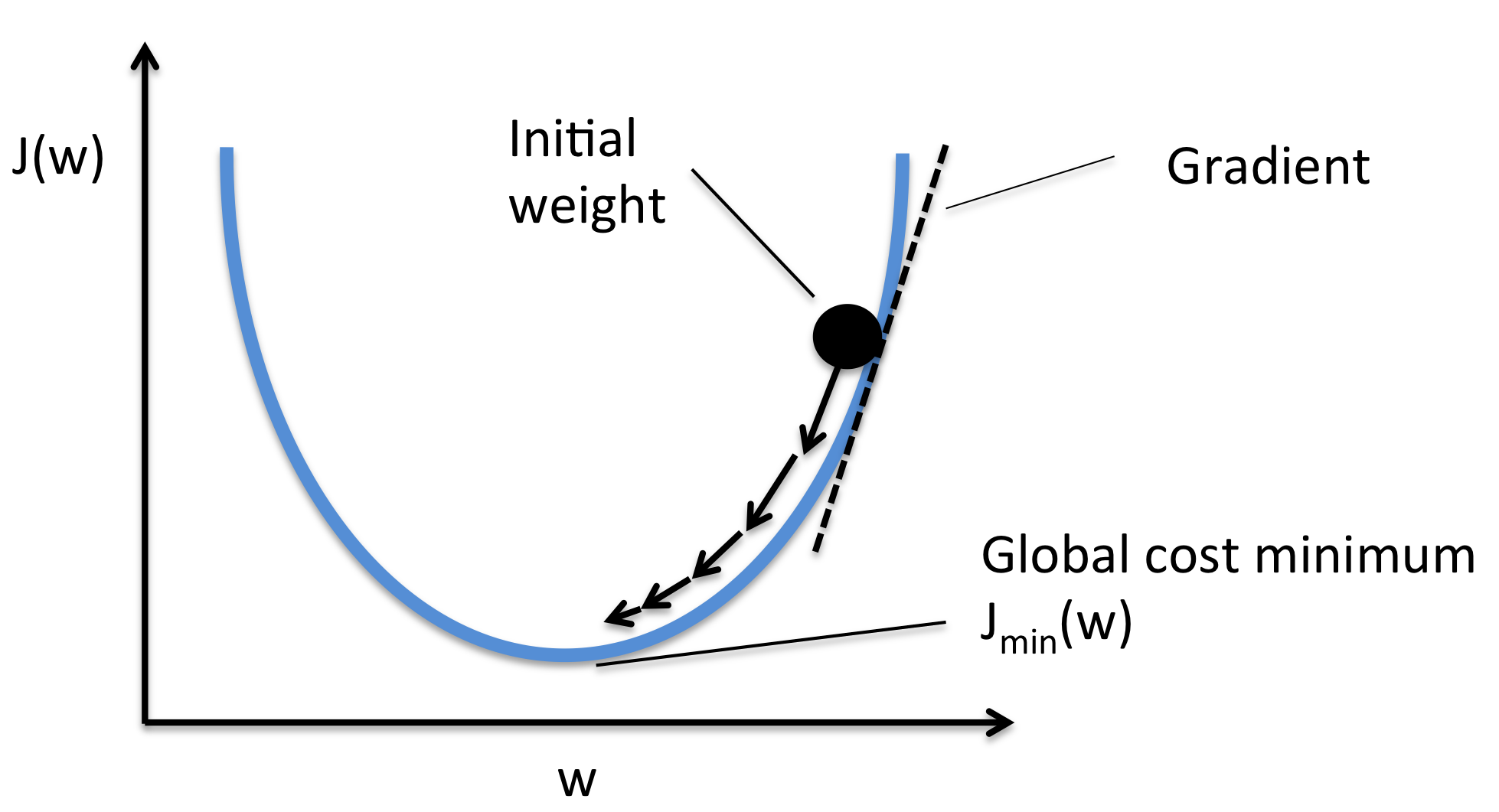
Gradient descent is a first order iterative optimization algorithm for finding the minimum of a function. To find a local minimum of a function using gradient descent, one takes steps proportional to the negative of the gradient of the function at the current point. If instead one takes steps proportional to the positive of the gradient, one approaches a local maximum of the function which is known as gradient ascent.
Gradient descent is based on the observation that if the multi-variable function (error or loss function) \(F(\mathbf{x})\) is defined and differentiable in a neighborhood of a point \(\mathbf{a}\), then \(F(\mathbf{x})\) decreases fastest if one goes from \(\mathbf{a}\) in the direction of the negative gradient of \(F\) at \(\mathbf{a}\), \(-\nabla F(\mathbf{a})\), where \(\gamma\) is the learning rate.
- Backpropagation
- Backpropagation process is carrying the error terms and updates parameters using gradient descent
- Gradient descent uses the gradient of error function \(F\) respect to the parameters.
- It updates the parameters in the opposite direction of the gradient of the loss function.
- Drawback of Gradient Descent
- The traditional batch gradient descent will calculate the gradient of the whole data set.
- But it will perform only one update, hence it can be very slow and hard to control for datasets which are very large and don’t fit in the memory.
- Also, it computes redundant updates for large data sets.
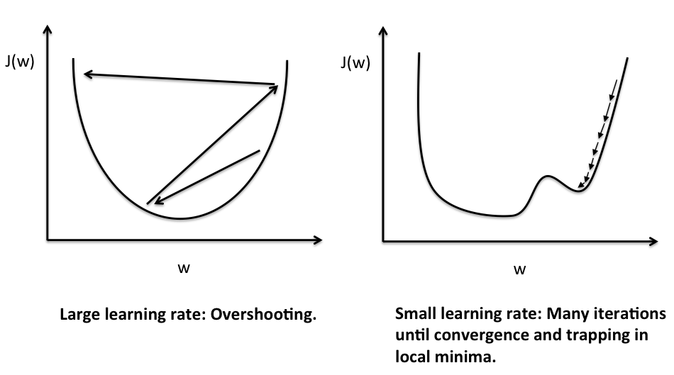
- Learning Rate
- Learning rate is an amount of decreasing function of each time.
- Large learning rate could make it bounce back and forth around the minimum.
- Small learning rate makes it search with a small step and converge very slow.
Stochastic Gradient Descent
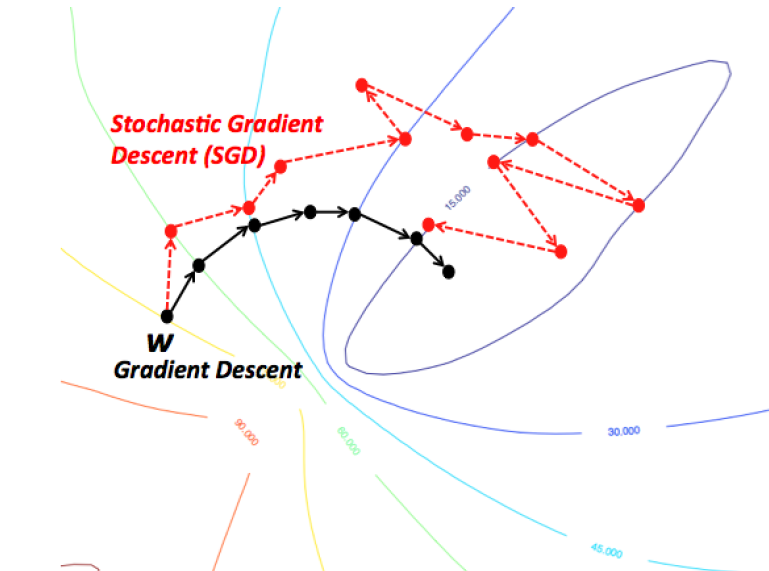
- Point: Stochastic gradient descent performs a parameter update for each training example \(x^i\) and label \(y^i\).
Stochastic gradient descent (SGD) is a stochastic approximation of the gradient descent and iterative method for minimizing an objective function. First SGD was used with each training example (one batch), but these days, we used mini-batch for better performance which is also called mini batch gradient descent.
- Motivation
- A recurring problem in machine learning is that large training sets are necessary for good generalization, but it cause more computationally expensive.
- The cost function often decomposes as a sum over training examples of some per-example loss function.
- The computational cost of below operation is \(O(m)\) which the time to take a single gradient step becomes prohibitively long as the training set size \(m\) grows.
- Insight
- The insight of SGD is that the gradient is an expectation.
- The expectation may be approximately estimated using a small set of samples.
- Specifically, on each step of the algorithm, we can sample a minibatch of examples drawn uniformly from the training set.
- The minibatch size \(m'\) is typically chosen to be a relatively small number of examples and it is usually held fixed as the training set size \(m\) grows.
- We may fit a training set with billions of examples using updates computed on only a hundred examples.
The estimate of the gradient using minibatch is formed as,
where \(\epsilon\) is the learning rate.
- Pros
- For a fixed model size, the cost per SGD update does not depend on the training set size \(m\).
- So, asymptotic cost of training a model with SGD is \(O(1)\) as a function of \(m\).
- It is much faster and performs one update at a time.
- Due to the frequent updates, parameters updates have high variance and causes the loss function to fluctuate to different intensities.
- This is actually a good thing because it helps us discover new and possibly better local minima, whereas standard gradient descent will only converge to the minimum of the basin.
- Mini-batch gradient descent is typically the algorithm of choice when training a neural network nowadays.
- Cons
- The problem of SGD is that due to the frequent updates and fluctuations, it ultimately complicates that convergence to the exact minimum and will keep overshooting.
- This can be solved by slowly decreasing the learning rate \(\epsilon\), SGD shows the same convergence pattern as standard gradient descent.
Challenges of Gradient Descent
- Choosing a proper learning rate is difficult.
- Small learning rate would give slow convergence.
- Large learning rate can hinder convergence and cause the loss function to fluctuate around the minimum or even to diverge.
- The same learning rate applies to all parameter updates.
- If our data is sparse and our features have very different frequencies, we might not want to update all of them to the same extent, but perform a larger update for rarely occurring features.
- Avoiding getting trapped in the numerous sub-optimal local minima and saddle point is hard while minimizing highly non-convex error functions.
- The saddle points are usually surrounded by a plateau of the same error, which makes it notoriously hard for SGD to escape, as the gradient is close to zero in all dimensions.
Optimizing the Gradient Descent
There are various algorithms further optimized gradient descent algorithm
Momentum
- Point: As SGD has trouble navigating ravines, Momentum accelerate SGD to converge in ravines.
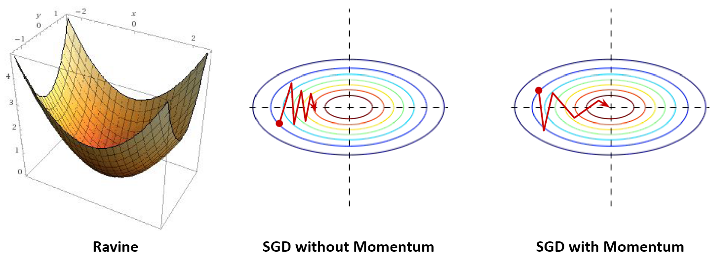
SGD has high variance oscillations and it makes hard to reach convergence, especially in ravines. In order to handle this problem, momentum is introduced to accelerate SGD by navigating along the relevant direction and softens the oscillations in irrelevant directions. SGD with momentum remembers the update \(\triangledown w\) at each iteration, and determines the next update as a linear combination of the gradient and the previous update.
that leads to:
where the parameter \(w\) which minimizes \(Q(w)\) is to be estimated, and \(\eta\) is learning rate. The momentum term \(\alpha\) increases for dimensions whose gradients point in the same directions and reduces updates for dimensions whose gradients change directions.
- Pros
- Unlike standard SGD, it tends to keep traveling in the same direction, preventing oscillations.
- It leads faster and stable convergence.
- Cons
- When it reach the minima, the momentum is usually high and it does not knows to slow down at that point which could cause to miss the minima entirely and continue to move up.
Nesterov Accelerated Gradient
- Point: As the momentum sometimes do not stop on the minima because of high momentum, NAG solve the problem by jumping based on the previous momentum first, and then calculate the gradient.
Nesterov Accelerated Gradient (NAG) solve the problem of momentum technique which could cause to miss the minima because of high momentum at the point. This technique first make a big jump based on the previous momentum then calculate the gradient and then make an correction which results in an parameter update. This anticipatory update prevents us to go too fast and not miss the minima and makes it more responsive to changes.
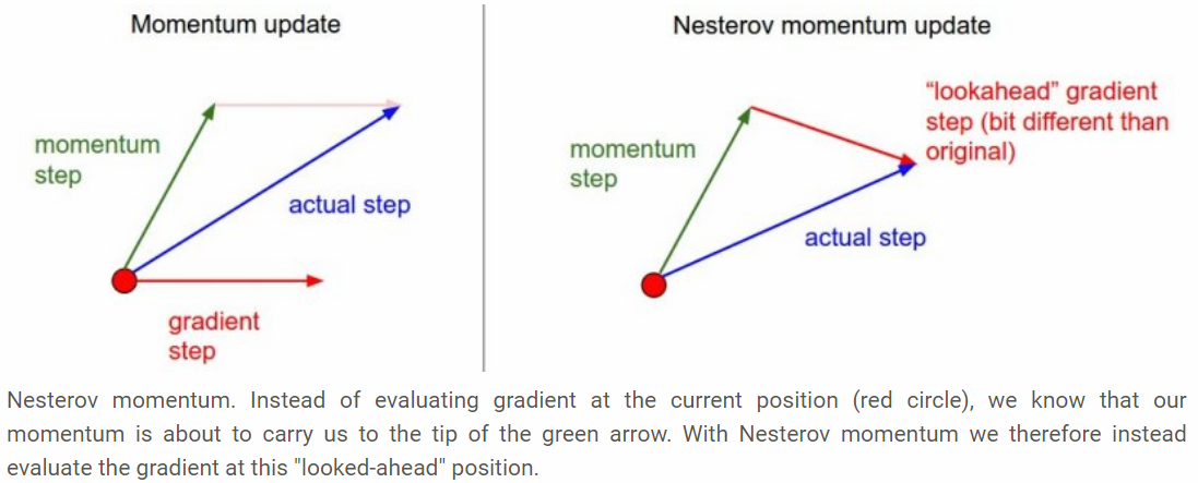
Computing \(w - \alpha \Delta w\) gives us an approximation of the next position of the parameters. We can look ahead by calculating the gradient not w.r.t. our current parameters \(w\) but w.r.t. the approximate future position of our parameters:
that leads to:
Algorithms with Adaptive Learning Rates
Adagrad
- Point: Adagrad adapts the learning rate to the parameters, performing larger updates for infrequent and smaller updates for frequent parameters.
Adagrad that maintains a per-parameter learning rate that improves performance on problems with sparse gradients (data). It increases the learning rate for more sparse parameters and decreases the learning rate for less sparse ones. This strategy often improves convergence performance over standard SGD in settings where data is sparse and sparse parameters are more informative. Examples of such applications include natural language processing and image recognition. It has a base learning rate \(\eta\), but this is multiplied with the elements of a vector \(G_{j,j}\) which is the diagonal of the outer product matrix.
where \(g_\tau = \nabla Q_i(w)\), the gradient, at iteration \(\tau\). The diagonal is given by
This vector is updated after every iteration. The formula for an update is now
or, written as per-parameter updates,
- Pros
- We do not need to manually tune the learning rate.
- Cons
- Its learning rate \(-\eta\) is always decreasing and decaying.
- This happens due to the accumulation of each squared gradients in the denominator, since every added term is positive.
- This causes the learning rate to shrink and eventually become so small, that the model just stops learning entirely.
- As the learning rate gets smaller and smaller, it gives very slow convergence.
Adadelta
- Point: Adadelta handled the decaying learning rate problem by restricting the window of accumulated past gradients to some fixed size.
Adadelta is an extension of Adagrad which handled the decaying learning rate problem of Adagrad. Instead of accumulating all previous squared gradients, adadelta limits the window of accumulated past gradients to some fixed size \(w\).
The sum of gradients is recursively defined as a decaying average of all past squared gradients. The running average \(E[g^2]_t\) at time step \(t\) then depends only on the previous average and the current gradient
\[E[g^2]_t = \gamma E[g^2]_{t-1} + (1 - \gamma) g^2_t\]We set \(\gamma\) to a similar value as the momentum term, around 0.9. For clarity, we now rewrite our vanilla SGD update in terms of the parameter update vector \(\Delta \theta_t\):
\[\begin{align} \begin{split} \Delta \theta_t &= - \eta \cdot g_{t, i} \\ \theta_{t+1} &= \theta_t + \Delta \theta_t \end{split} \end{align}\]The parameter update vector of Adagrad that we derived previously thus takes the form:
\[\Delta \theta_t = - \dfrac{\eta}{\sqrt{G_{t} + \epsilon}} \odot g_{t}\]We now simply replace the diagonal matrix \(G_t\) with the decaying average over past squared gradients \(E[g^2]_t\):
\[\Delta \theta_t = - \dfrac{\eta}{\sqrt{E[g^2]_t + \epsilon}} g_{t}\]As the denominator is just the root mean squared (RMS) error criterion of the gradient, we can replace it with the criterion short-hand:
\[\Delta \theta_t = - \dfrac{\eta}{RMS[g]_{t}} g_t\]- Pros
- Removed the decaying learning rate problem of AdaGrad
- We do not need to set a default learning rate.
RMSProp
- Point: RMSProp also handled the decaying learning rate problem of Adagrad that is identical to the first update vector of Adadelta.
Root Mean Square Propagation (RMSProp) that also maintains per-parameter learning rates that are adapted based on the average of recent magnitudes of the gradients for the weight (e.g. how quickly it is changing). This means the algorithm does well on online and non-stationary problems (e.g. noisy).
\[\begin{align} \begin{split} E[g^2]_t &= 0.9 E[g^2]_{t-1} + 0.1 g^2_t \\ \theta_{t+1} &= \theta_{t} - \dfrac{\eta}{\sqrt{E[g^2]_t + \epsilon}} g_{t} \end{split} \end{align}\]Adam
- Point: Adam is an adaptive learning rate method and also storing an exponentially decaying average of past squared gradient like Adadelta and RMSprop.
Adaptive Moment Estimation (Adam) is another method that computes adaptive learning rates for each parameter which is combination between Adagrad and RMSprop. In addition to storing an exponentially decaying average of past squared gradients \(v_t\) like Adadelta and RMSprop, Adam also keeps an exponentially decaying average of past gradients \(m_t\), similar to momentum:
\[\begin{align} \begin{split} m_t &= \beta_1 m_{t-1} + (1 - \beta_1) g_t \\ v_t &= \beta_2 v_{t-1} + (1 - \beta_2) g_t^2 \end{split} \end{align}\]\(m_t\) and \(v_t\) are estimates of the first moment (the mean) and the second moment (the uncentered variance) of the gradients respectively. As \(m_t\) and \(v_t\) are initialized as vectors of 0’s, the authors of Adam observe that they are biased towards zero, especially during the initial time steps, and especially when the decay rates are small.
They counteract these biases by computing bias-corrected first and second moment estimates:
\[\begin{align} \begin{split} \hat{m}_t &= \dfrac{m_t}{1 - \beta^t_1} \\ \hat{v}_t &= \dfrac{v_t}{1 - \beta^t_2} \end{split} \end{align}\]They then use these to update the parameters just as we have seen in Adadelta and RMSprop, which yields the Adam update rule:
\[\theta_{t+1} = \theta_{t} - \dfrac{\eta}{\sqrt{\hat{v}_t} + \epsilon} \hat{m}_t\]The authors propose default values of 0.9 for \(\beta_1\), 0.999 for \(\beta_2\), and \(10^{-8}\) for \(\epsilon\). They show empirically that Adam works well in practice and compares favorably to other adaptive learning-method algorithms.
AdamW
After the Adam optimizer was introduced, few studies began to discourage to us Adam and showed several experiments that SGD with momentum is performing better. In the end of 2017, Ilya Loshchilov and Frank Hutter announced improved version of Adam optimizer in the paper The Marginal Value of Adaptive Gradient Methods in Machine Learning. They pointed out that the way weight decay is implemented in Adam in every library seems to be wrong and proposed a way to fix it called AdamW.
The main contributions of the AdamW paper is to improve Adam’s performance:
- Decoupling weight decay from the gradient-based update
- The author suggest to use the original formulation of weight decay to decouple the gradient-based update from weight decay.
- Normalizing the values of weight decay
- The author propose to parameterize the weight decay factor as a function of the total number of batch passes.
- This leads to a better invariance of the hyperparameter settings.
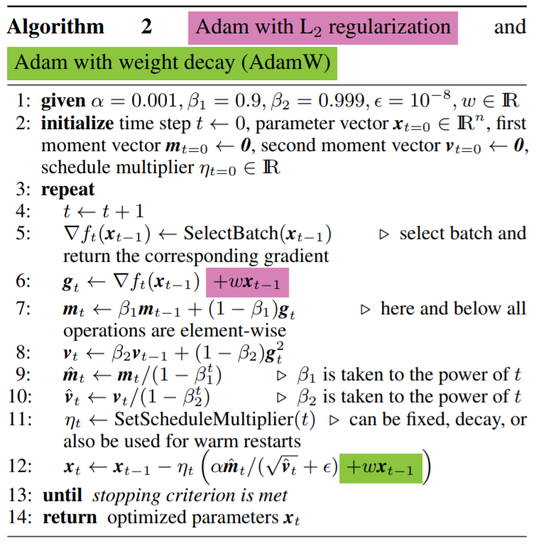
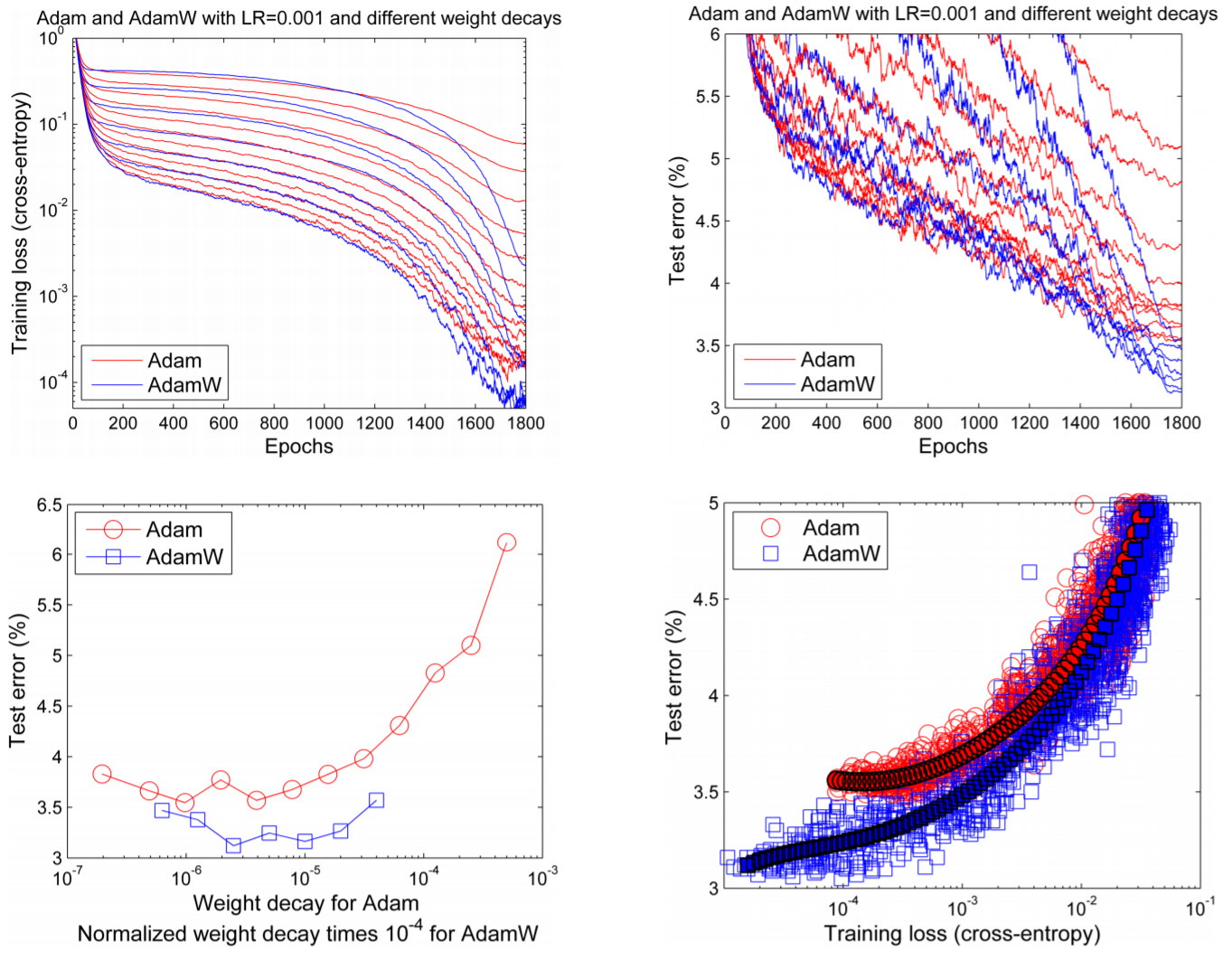
Figure: Learning curves (top row) and generalization results (bottom row) obtained by a 26 2x96d ResNet trained with Adam and AdamW on CIFAR-10. See text for details. SuppFigure 5 (supplemental material) shows the same qualitative results for ImageNet32x32.
Visualization of Algorithms
As shown in below images, the adaptive learning-rate methods, i.e. Adagrad, Adadelta, RMSprop, and Adam are most suitable and provide the best convergence for these scenarios.
- In the below image, we see their behaviour on the contours of a loss surface over time.
- Note that Adagrad, Adadelta, and RMSprop almost immediately head off in the right direction and converge similarly fast, while Momentum and NAG are led off-track,
- NAG, however, is quickly able to correct its course due to its increased responsiveness by looking ahead and heads to the minimum.
- In the below image, it shows the behaviour of the algorithms at a saddle point.
- Notice here that SGD, Momentum, and NAG find it difficulty to break symmetry.
- Although the two latter eventually manage to escape the saddle point, while Adagrad, RMSprop, and Adadelta quickly head down the negative slope.
Which Optimizer to Use?
- If the input data is sparse, then using one of the adaptive learning rate methods will give the best results.
- One benefit of using them is that you would not need to tune the learning rate.
- If you want fast convergence and train a deep or complex network, choose one of the adaptive learning rate methods.
- Adam works well in practice and outperforms other adaptive techniques.
- Some people say Adam does not generalize as well as SGD with Momentum.
- Usually, it is because of choosing poor hyperparameters.
- Adam generally requires more regularization than SGD, so make sure to adjust regularization hyper-parameters.
References
- Book: Deep Learning book [Link]
- Blog: Types of Optimization Algorithms used in Neural Networks and Ways to Optimize Gradient Descent [Link]
- Wikipedia: Gradient [Link]
- Wikipedia: Gradient Descent [Link]
- Wikipedia: Stochastic gradient descent [Link]
- Web: CS231n Convolutional Neural Networks for Visual Recognition [Link]
- Blog: An overview of gradient descent optimization algorithms[Link]
- Paper: Fixing Weight Decay Regularization in Adam
- Paper: The Marginal Value of Adaptive Gradient Methods in Machine Learning