Research on several vision techniques such as pixel difference and optical flow.
Pixel Difference
- A pixel difference algorithm is a straightforward method to calculate the visual difference between two frames.
- Based on absolute pixel-wise intensity differences,
- Where \(m\) and \(n\) are the pixel number in horizontal and vertical dimensions of a frame respectively
- And \(f(i,j)\) is the pixel intensity at \((i,j)\) which is a single number that represents the brightness of the pixel
- An index of visual difference is defined by:
\[D(f_1, f_2)=\frac{1}{m*n}\sum_{i=0}^{m-1}\sum_{j=0}^{n-1}\mid f_1(i,j)-f_2(i,j)\mid\]
- The other algorithm for counting the total number of pixels that have a greater change value than the threshold value \(s\) is defined by:
\[DP(i,j) = \left\{
\begin{aligned}
1 \qquad if \mid f_1(i,j)-f_2(i,j) \mid > s \\
0 \qquad if \mid f_1(i,j)-f_2(i,j) \mid \leq s
\end{aligned}
\right.\]
- Usually, pixel-wise difference algorithms are very sensitive to noise and camera motion.
- Improvement can be achieved by dividing the image into sub-regions and comparing at the region level.
- The second limitation is the sensitivity to illumination.
- Some normalization technique (e.g. using histogram) can overcome parts of the illumination effects.
Pixel-Based Statistical Difference
- Pixel-based statistical difference algorithms treat the pixel-wise intensity as a distribution and the difference of two frames within a shot as two distribution coming from the same population.
- That means there is no statistically significant difference for two consecutive frames that come from a single shot.
- Theoretically, any statistical approach to test whether two distributions come from the same population can be applied in shot detection.
- To improve accuracy, a frame is divided into several regions and an index based on the mean and standard deviation of intensity values of pixels in the corresponding regions is calculated in order to determine the similarity.
- Where \(m\) is the mean intensity, \(\sigma\) is the variance, and \(r\) is the region, the similarity is defined by:
\[D_r = \frac{[(\frac{\sigma_1^2+\sigma_2^2}{2})+(\frac{m_1^2-m_2^2}{2})]^2}{\sigma_1^2\sigma_2^2}\]
Optical Flow
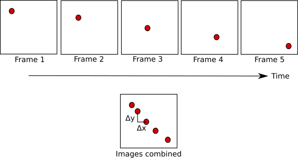
- Optical Flow is the pattern of apparent motion of objects, surfaces, and edges in a visual scene caused by the relative motion between an observer and a scene.
- The feature is tracked from frame to frame and the output is the distance that the feature moved since the previous frame.
- It describes the direction and the speed of the motion of features in an image.
- The computation is based on two assumptions:
- The observed brightness of any object point is constant over time.
- Neighboring pixels in the image plain move in a similar manner.
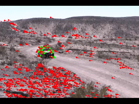
Lucas-Kanade Method
- Lucas-Kanade method is a widely used differential method for optical flow estimation in computer vision.
- It assumes that the flow is essentially constant in a local neighbourhood of the pixel under consideration.
- And it solves the basic optical flow equations for all the pixels in that neighbourhood, by the least squares criterion.
- It sets each pixel window of one frame and finds the best match with this window in the next frame.
- Pros
- By combining information from several nearby pixels, the Lucas-Kanade method can often resolve the inherent ambiguity of the optical flow equation.
- It is also less sensitive to image noise than point-wise methods.
- Cons
- Because it uses a small local window, there is a disadvantage that the movement can not be calculated if the movement is larger than the window.
- It cannot provide flow information in the interior of uniform regions of the image, since it is a purely local method.