“Gradient Acceleration in Activation Functions” argues that the dropout is not a regularizer but an optimization technique and propose better way to obtain the same effect with faster speed. The authors are Sangchul Hahn and Heeyoul Choi from Handong Global University.
Summary
- Research Objective
- To propose a new explanation of why dropout works and propose a new technique to design better activation functions.
- Proposed Solution
- The author claims that dropout is an optimization technique to push the input towards the saturation area of nonlinear activation function by accelerating gradient information flowing even in the saturation area in backpropagation.
- Propose a new technique for activation functions, gradient acceleration in activation function (GAAF), that accelerates gradients to flow even in the saturation area.
- Then, input to the activation function can climb onto the saturation area which makes the network more robust because the model converges on a flat region.
- Contribution
- Proved that dropout is an effective optimization technique to generate more gradient information flowing through the layers so that it pushes the nets towards the saturation areas of nonlinear activation functions.
- Proposed GAAF that accelerates gradient information in a deterministic way, so that it has the similar effect to the dropout method, but with less iterations.
Dropout Analysis
Dropout
Dropout was proposed in Hinton et al. (2012) to prevent co-adaptation among the hidden nodes of deep feed forward neural networks.
- It randomly drops out hidden nodes with probability \(p\) druing training step.
- In the test phase, the nodes of the model are rescaled by multiplying \((1-p)\), which has the effect of taking the geometric mean of \(2^N\) dropped-out models.
In this paper, the author question the conventional explanation about dropout, and argue that dropout is an effective optimization technique, which does not avoid co-adaptation. In addition, dropout usually takes much more time to train neural networks, so the author propose a new activation function which is no need for dropout.
Co-adaptation
In Figure 1, In both networks, the top layer (Layer 3) looks more of the Gaussian distribution which indicates that the top layer trained more than the lower layers. Dropout makes the three distribution Gaussian-like with similar statistics. This implies that the lower layers are trained more with dropout than without dropout, which is turn implies that gradient information flows more into the lower layer with dropout.
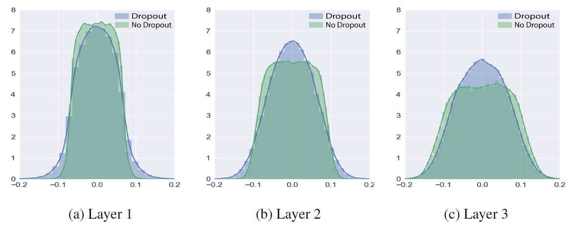 Figure 1: Distributions of the weights in each layer after training the models on MNIST. The bars indicate normalized histogram and the solid curves are drawn by kernel density estimation. Layer 1 is the bottom layer.
Generally, correlation between node values is a necessary condition for co-adaptation of the nodes.
In Figure 2, the nodes trained with dropout have higher correlations than the nodes trained without dropout, which is against the conventional explanation for dropout.
Based on the results, the authors argue that dropout does not avoid co-adaptation.
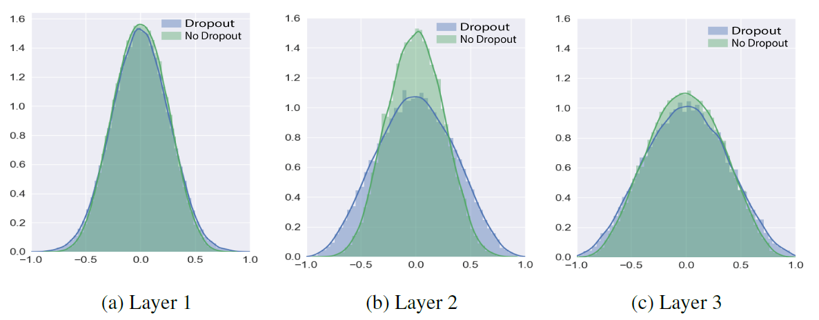 Figure 2: Comparison of distribution of node correlation after training two models on MNIST.
Optimization
If dropout does not avoid co-adaptation, then what can explain the performance improvement by dropout? The author argues that dropout generates more gradient information though layers as an optimization technique. Table 2 summarizes that dropout increases the amount of gradient information flowing, which is around five times.
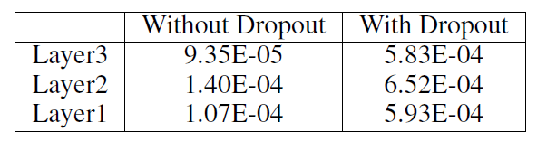 Figure 3: The amount of gradient information flowing through layers during training. The values in the table are the average value of the absolute value of gradient of all nodes in each layer during the whole iterations.
Gulcehre et al. 2016 shows that the noise allows gradients to flow easily even when the net is in the saturation ares. Likewise, dropout could increase the amount of gradient in a similar way.
Dropout makes a significant variance for the net, due to the randomness of \(d_i\):
\[Var(\sum^{N}_{i}w_i d_i x_i) > 0\]The variance of the net values increases chances to have more gradient information especially around the boundary of saturation areas. In Figure 4, when the derivative is almost zero without dropout, there is no gradient flowing through the node. However, if it has a variance, \(z_i\) can randomly move to the right or left. If it goes left, it obtains gradient information which is generated by dropout with certain amount of probability. The author argues that it is the main reason of the dropout effect.
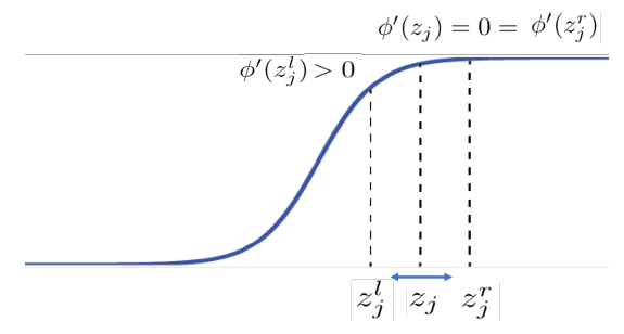 Figure 4: Variance in the saturation area increases the probability to have gradient information, by which dropout generates gradients.
To see whether dropout actually pushes the net values towards the saturation areas, the author checked the node value distributions with test data after training. Figure 4 shows that the model trained with dropout has more net values in the saturation area of tanh, which is critical to have better generalization for test data. The higher layer has more net values in the saturation area, since the variance of the lwer layers are transfered to the higher layer.
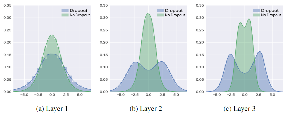 Figure 5: Distributions of net values to tanh for the MNIST test data.
Gradient Acceleration in Activation Function
As dropout takes a lot of time to train, the author suggest gradient acceleration in activation function (GAAF) which directly add gradient information for the backpropagation, while not changing the output values for the forward-propagation.
Given a nonlinear activation function, \(\phi(x)\), the author modifyies it by adding a gradient acceleration function, \(g(\cdot)\) which is defined by:
\[g(x) = (x*K- \lfloor x*K \rfloor - 0.5)/K\]- Notation
- \(\lfloor \cdot \rfloor\) is the floor operation
- \(K\) is frequency constant (10,000 in experiments)
\(g(x)\) is almost zero (\(<\frac{1}{K}\)) but the gradient of \(g(x)\) is 1 almost everywhere, regardless of the input value \(x\). The difference between \(\phi(x)\) and the new function \(\phi(x)+g(x)\) is less than \(\frac{1}{K}\), which is negligible.
As dropout does not generate gradient information on the leftmost or rightmost saturation areas, the author also decreases the gradient acceleration on those areas by multiplying a shape function \(s(\cdot)\) to \(g(\cdot)\).
\[\phi_{new}(x) = \phi(x)+g(x)*s(x)\]where \(s(\cdot)\) needs to be defined properly depending on the activation function, \(\phi(\cdot)\). For example, when \(\phi\) is \(tanh\) or \(ReLU\), an exponential function or a shifted sigmoid function can work well as \(s(\cdot)\), respectively.
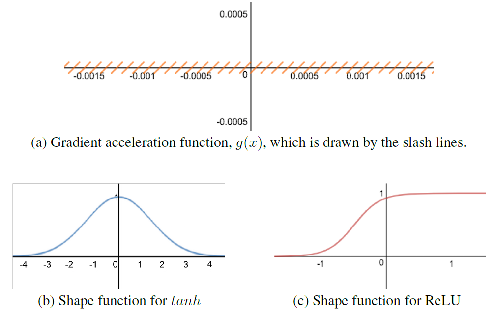 Figure 6: (a) Gradient acceleration function, and (b,c) two shape functions for two activation functions.
The proposed gradient acceleration function \(g(\cdot)\) generates gradients in a deterministic way, while dropout generates gradient stochastically based on the net variances. Thus, GAAF has the same effect as dropout but it converges faster than dropout. If the rate of dropout decreases, then the net variance would decrease, which in turn decreases the amount of grdient. To obtain the same effect with GAAF, the shape function needs to be reshaped according to the dropout rate.
Experiments
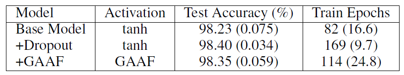 Figure 7: Experiment results on MNIST. The accuracies and epochs are the average values of five executions. The numbers in the parentheses are the corresponding standard deviations.
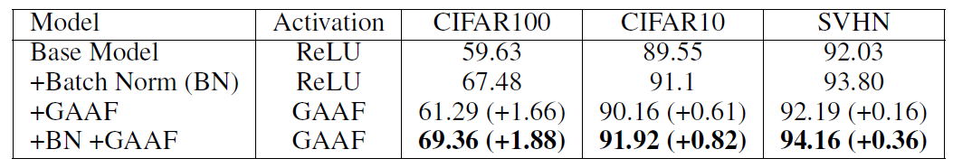 Figure 8: Test accuracies (%) on CIFAR and SVHN. The numbers are Top-1 accuracies. The improvements achieved by GAAF are presented in the parentheses.