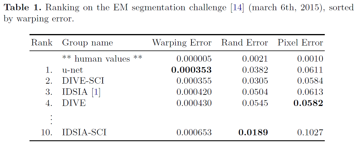
“U-Net: Convolutional Networks for Biomedical Image Segmentation” is a famous segmentation model not only for biomedical tasks and also for general segmentation tasks, such as text, house, ship segmentation.
Summary
- Proposed Solution
- Present a network and training strategy that relies on the strong use of data augmentation to use the available annotated samples more efficiently.
- The architecture consists of a contracting path to capture context and a symmetric expanding path that enables precise localization.
- Contribution
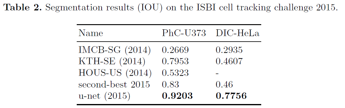
- U-net can be trained end-to-end from very few images and outperforms the prior best method on the ISBI challenge for segmentation of neuronal structures in electron microscopic stacks.
- It is fast, segmentation of a 512x512 image takes less than a second on a recent GPU.
U-Net
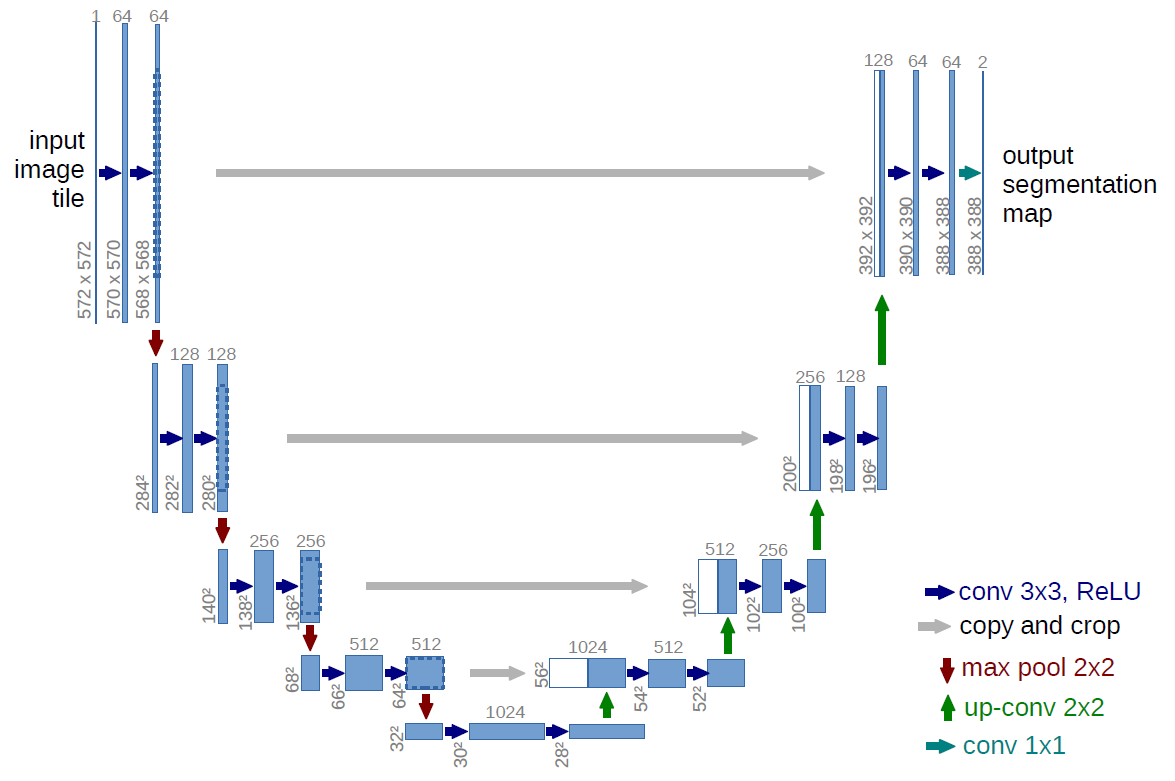
Figure 1: U-net architecture(example for 32x32 pixels in the lowest resolution). Each blue box corresponds to a multi-channel feature map. The number of channels is denoted on top of the box. The x-y-size is provided at the lower left edge of the box. White boxes represent copied feature maps. The arrows denote the different operations.
Network Architecture
U-net consits of a contracting path (left side) and an expansive path (right side).
- Contracting path
- typical architecture of a convolutional network
- repeated application of two 3x3 convolutions (unpadded convolutions)
- each followed by a rectified linear unit (ReLU) and a 2x2 max pooling operation with stride 2 for downsampling
- at each downsampling step, we double the number of feature channels
- Expansive path
- consists of an upsampling of the feature map followed by a 2x2 convolution (“up-convolution”) that halves the number of feature channels
- a concatenation with the correspondingly cropped feature map from the contracting path, and two 3x3 convolutions
- each followed by a ReLU
- the cropping is necessary due to the loss of border pixels in every convolution
At the final layer a 1x1 convolution is used to map each 64-component feature vector to the desired number of classes. In total the network has 23 convolutional layers.
Training
The energy function is computed by a pixel-wise soft-max over the final feature map combined with the cross entropy loss function. The soft-max is defined as
\[p_k(x)=exp(a_k(x))/(\sum_{k'=1}^Kexp(a_{k'}(x)))\]The cross entropy then penalizes at each position the deviation of \(p_{l(x)}(x)\) from 1 using
\[E = \sum_{x\in Ω}w(x)log(p_{l(x)}(x))\]The seperation border is computed using morphological operations. The weight map is then computed as
\[w(x) = w_c(x) + w_0 \cdot exp(-\frac{(d_1(x)+d_2(x))^2}{2\sigma^2})\]Experiments