Learn the basics about Recurrent Neural Network (RNN), its detail and case models of RNN.
Recurrent Neural Network (RNN)
What is RNN?
- Recurrent Neural Network is a network with loops in it for allowing information to persist.
- Traditional neural network could not reason about previous events to inform later ones.
- RNN address this issue by having loops as the figure below (an unrolled RNN).
- A loop in a chunk of neural network \(A\) allows information to be passed from one step to the next.

The Process of Carrying Memory Forward Mathematically
\[h_t = f(h_{t-1}, x_t)\\
\hspace{6em} = f(W_{hh}h_{t-1} + W_{xh}x_t)\\\]
- \(h_t\): the new state, \(h_{t-1}\): the previous state while \(x_t\) is the current input.
- \(W_{xh}\): the weight at the input neuron, \(W_{hh}\): the weight at the recurrent neuron (known as a transition matrix and similar to a Markov chain)
- The weight matrices are filters that determine how much importance to accord to both the present input and the past hidden state.
- The error they generate will return via backpropagation and be used to adjust their weight.
- \(f()\): activation function, either a logistic sigmoid or tanh
- Which is a standard tool for condensing very large or very small values into a logistic space, as well as making gradients workable for backpropagation.
Backpropagation Through Time (BPTT)
- In case of a backward propagation in RNN, it goes back in time to change the weights, which is called Back Propagation Through Time (BPTT).
- The error is calculated as a cross entropy loss:
- \(y_t\): the predicted value, \(\bar{y}_t\): the actual value
\[E_t(\bar{y}_t, y_t) = -\bar{y}_t \log(y_t)\\
E(\bar{y}, y) = -\sum\bar{y}_t \log(y_t)\\\]
- Steps for backpropagation
- The cross entropy error is first computed using the current output and the actual output.
- Remember that the network is unrolled for all the time steps.
- For the unrolled network, the gradient is calculated for each time step with respect to the weight parameter.
- Now that the weight is the same for all the time steps the gradients can be combined together for all time steps.
- The weights are then updated for both recurrent neuron and the dense layers.
- Truncated BPTT
- Truncated BPTT is an approximation of full BPTT that is preferred for long sequences, since full BPTT’s forward/backward cost per parameter update becomes very high over many time steps.
- The downside is that the gradient can only flow back so far due to that truncation, so the network can’t learn dependencies that are as long as in full BPTT.
Vanishing and Exploding Gradients
Because the layers and time steps of deep neural networks relate to each other through multiplication, derivatives are susceptible to vanishing or exploding. Let’s define \(h_t\) of RNN as,
\[h_{t}=tanh(W_{hh}h_{t-1} + W_{xh}X_{t} + b_{h})\]
When we compute derivative of \(h_T\) with respect to \(h_t\) \((T>t)\), it can be defined by using chain rule,
\[\frac{\partial h_{T}}{\partial h_{t}} =
\frac{\partial h_{T}}{\partial h_{T-1}} *
\frac{\partial h_{T-1}}{\partial h_{T-2}} *
... *
\frac{\partial h_{t+1}}{\partial h_{t}}, \\
\frac{\partial h_{T}}{\partial h_{T-1}}=W_{hh}*tanh'(W_{hh}h_{T-1} + W_{xh}X_{T} + b_{h}) \\
\frac{\partial h_{T-1}}{\partial h_{T-2}}=W_{hh}*tanh'(W_{hh}h_{T-2} + W_{xh}X_{T-1} + b_{h}) \\
... \\
\frac{\partial h_{t+1}}{\partial h_{t}}=W_{hh}*tanh'(W_{hh}h_{t} + W_{xh}X_{t+1} + b_{h})\]
So, it can be,
\[\frac{\partial h_{T}}{\partial h_{t}}=W_{hh}^{T-t}*\prod_{i=t}^{T-1}{tanh'(W_{hh}h_{i} + W_{xh}X_{i+1} + b_{h})}\]
- Exploding gradient
- The gradients will be exploded if the gradient formula is deep (large \(T-t\)) and a single or multiple gradient values becoming very high (if \(W_{hh} > 1\)).
- This is less concerning than vanishing gradient problem because it can be easily solved by clipping the gradients at a predefined threshold value.
- Vanishing gradient problem
- The gradients will be vanished if the gradient formula is deep (large \(T-t\)) and a single or multiple gradient values becoming very low (if -1 < \(W_{hh} < 1\)).
- Calculating the error after several time step with respect to the first one, there will be a long dependency.
- If any one of the gradients approached 0, all the gradient would rush to zero exponentially fast due to the multiplication of chain rule.
- This state would no longer help the network to learn anything which is known as vanishing gradient problem.
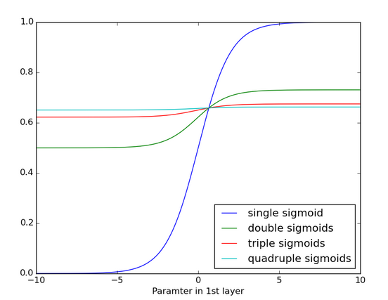
- Below is the effects of applying a sigmoid function over and over again, it became very flattened with no detectable slope where its gradient become close to 0.
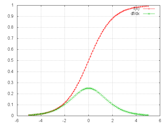
- Tanh is better than Sigmoid
- Since the RNN is sensitive by vanishing gradient problem, it is better to use activation function which can last gradient longer.
- In the Sigmoid figure below, it will be vulnerable because the maximum of \(dSigmoid(x)/dx\) is about 0.25.
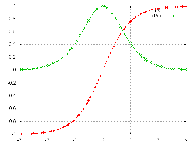
- In the Tanh figure below, it will be better than Sigmoid because the maximum of \(dtanh(x)/dx\) is about 1.
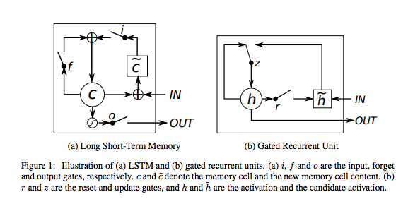
Long Short-Term Memory Unit (LSTM)
What is LSTM?
- LSTM help preserve the error that can be backpropagated through time and layers.
- Gradient vanishing happened because error \(\delta\) is multiplied by scaling factors \(\delta_i = \sigma '(y_i)W_{ji}\delta_j\) (connection from unit i to j)
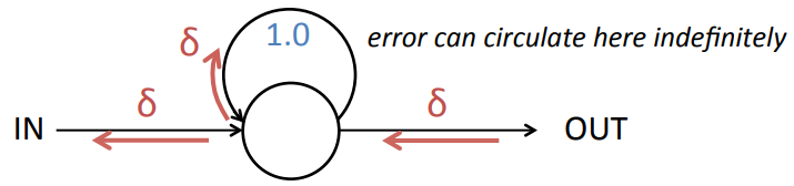
- LSTM overcomes this problem by having Constant Error Carrousel (CEC).
- CEC enables error propagation of arbitrary time steps by setting \(W_{ii}=1\) and \(\sigma(x)=x\).
- CEC with input gate and output gate is LSTM unit.
- Gates are for controlling error flow depending on the context.
- Forget gates is LSTM variants which explicitly reset the value in CEC.
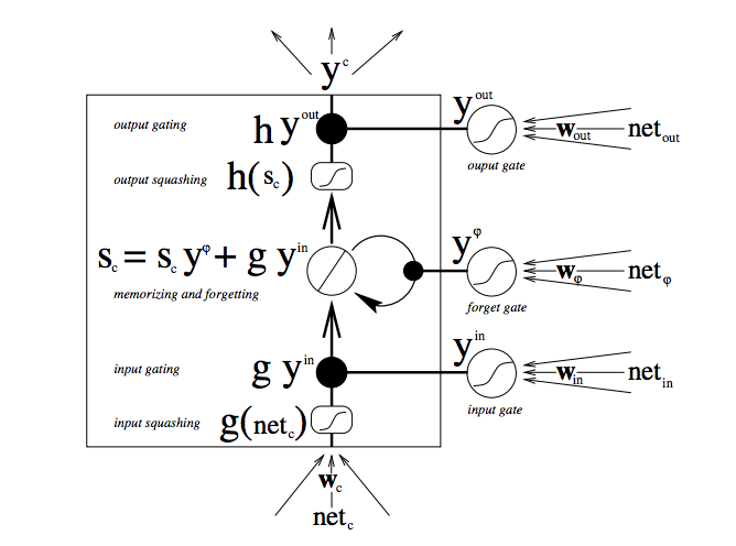
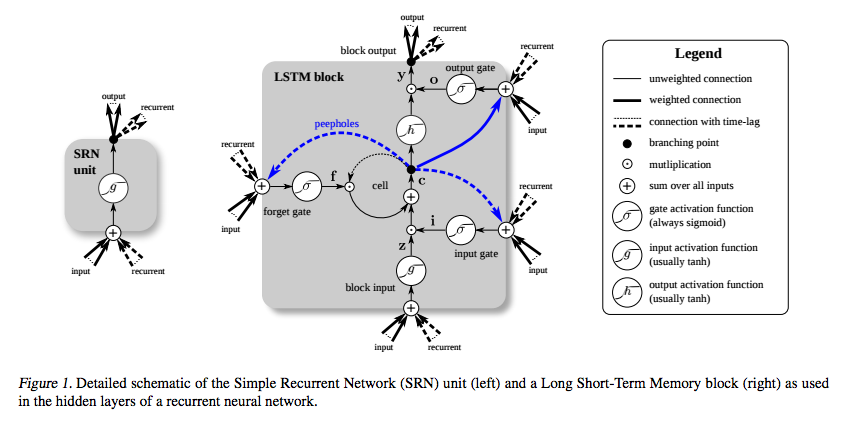
- LSTM architecture
- Information can be stored in, written to, or read from a cell.
- The cell makes decisions about what to store, and when to allow reads, writes and erasures, via gates that open and close.
- This is done by opening or shutting each gate and recombine their open and shut states at each steps.
- These gates are analog with the range 0-1 and have the advantage over digital of being differentiable, and therefore suitable for backpropagation.
- The figure below shows how data flows through a memory cell and is controlled by its gates
Comparison between RNN and LSTM
- LSTM’s memory cells give different roles to addition and multiplication in the transformation of input.
- The central plus sign helps them preserve a constant error when it must be backpropagated at depth.
- Instead of determining the subsequent cell state by multiplying its current state with new input, they add the two and that makes the difference.
Gated Recurrent Unit (GRU)
- A gated recurrent unit (GRU) is basically an LSTM without an output gate, which therefore fully writes the contents from its memory cell to the larger net at each time step.