Regularization

Regularization is important technique for preventing overfitting problem while training a learning model.

Regularization

Regularization is a way to prevent overfitting and get a model generalizes the data. Overfitting problem usually caused by large weight value \(W\), so common way of regularization is to simply adds the bigger penalty as model complexity increases. Regularization parameter \(\lambda\) penalizes all the parameters except intercept so that it will decrease the importance given to higher terms and will bring the model towards less complex equation.

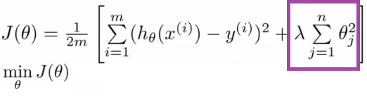Figure 1: Example of cost function with regularization term.

L1/L2 Regularization

L1 Regularization

L1 Regularization also called Lasso Regression adds absolute value of magnitude of coefficient as penalty term to the loss function. If \(\lambda\) is zero, it will be the same with original loss function. If \(\lambda\) is very large, it will add too much weight and it will lead to under-fitting. So, it is important how \(\lambda\) is chosen.

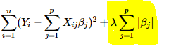Figure 2: L1 regularization.

L2 Regularization (weight decay)

L2 Regularization also called Ridge Regression is one of the most commonly used regularization technique. It adds squared magnitude of coefficient as penalty term to the loss function. If \(\lambda\) is zero, it will be the same with original loss function. If \(\lambda\) is very large, it will add too much weight and it will lead to under-fitting. So, it is important how \(\lambda\) is chosen as well.

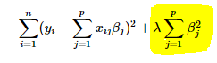Figure 3: L2 regularization.

Simply thinking that we add \(\frac{1}{2}\lambda W^2\) on the loss function and after computing gradient descent, \(W\) will be updated by,

\[W \leftarrow W - \eta(\frac{\partial L}{\partial W} + \lambda W)\]

So, \(\lambda W\) will work as penalty according to the amount of \(W\).

Dropout

Dropout [N. Srivastava et al., 2014] is one of the simplest and the most powerful regularization techniques. It prevents units from complex co-adapting by randomly dropping units from the network.

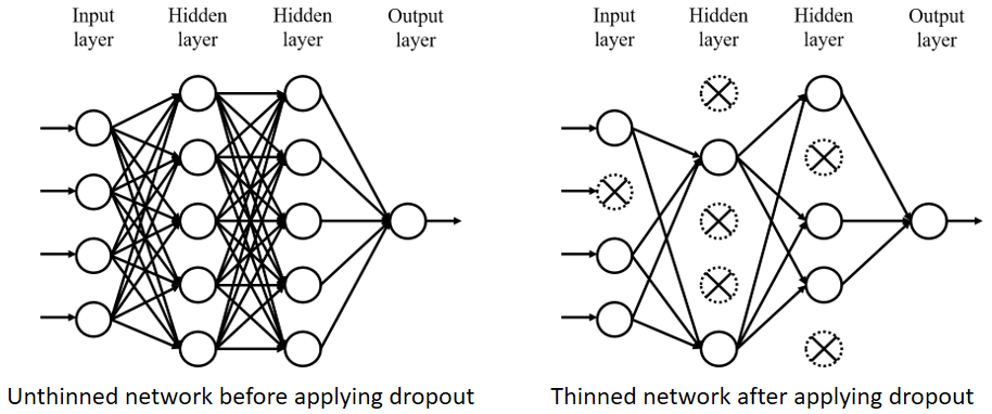
Figure 4: Comparison between network with dropout and without dropout.

• In the training stage
  • It randomly drops units using dropout rate
  • It has the effect of sampling a large number of different thinned networks.
  • Dropout rate: probability that a unit will be retained.
    • Optimal dropout rate is suggested around 0.5 in hidden layers and close to 1 for in input layer.
    • As it is a hyperparameter, it can be decided empirically.
• In the inference stage
  • A single unthinned network is used (no dropout applied)
  • Weights of the unthinned network has to be multiplied by the dropout rate to keep the output the same as training stage.
  • It approximates the effect of averaging the predictions of all thinned networks from the training process. (as ensemble learning)
• Drawbacks of dropout
  • It increases training time because of noisy parameter updates caused when each training step tries to train a different architecture.

Label Smoothing

Most datasets have some amount of mistakes in the labels and it makes minimizing cost function be harsh. One way to handle this is to explicitly model the noise on labels. This is done through setting a probability \(\epsilon\) for which it thinks the labels are correct. This probability is easily incorporated into the cross entropy cost function anlytically. Label smoothing is an example of this.

• Output vectors provided
  • \[y_{label} = [1,0,0, \cdots]\]
• Softmax output form
  • \[y_{out}=[0.87,0.001,0.04,\cdots]\]
• Label smoothing replaces the label vector with
  • \[y_{label}=[1-p,\frac{\epsilon}{K-1},\frac{\epsilon}{K-1},\cdots]\]
  • It prevents the pursuit of hard probabilities without discouraging correct classification.
• Label smoothing estimates the marginalized effect of label noise during training.
  • When the prior label distribution is uniform, label smoothing is equivalent to adding the KL divergence between the uniform distribution \(u\) and the network’s predicted distribution \(p_\theta\) to the negative log-likelihood.

\[\mathcal{L}(\theta)=-\sum \log p_\theta (y\mid x)-D_{KL}(u \parallel p_\theta(y \mid x))\]

Examples

• Regularizing neural networks by penalizing confident output distributions, ICLR2017
  • Paper
  • Proposed better regularization by connecting a maximum entropy based confidence penalty to label smoothing through the direction of the KL divergence
• Rethinking the Inception Architecture for Computer Vision, CVPR2016, Google
  • Used label-smoothing regularization (LSR) to encourage the model having less confidence so that it can avoid overfitting and increase the ability of the model to adapt.

References

• Blog: L1 and L2 Regularization Methods [Link]
• Paper: Dropout: A Simple Way to Prevent Neural Networks from Overfitting [Link]
• Slide: Regularizatino for deep models, University of Waterloo