Learn about probability which are the basics of artificial intelligence and deep learning.
Probability
Two Perspectives of Machine Learning
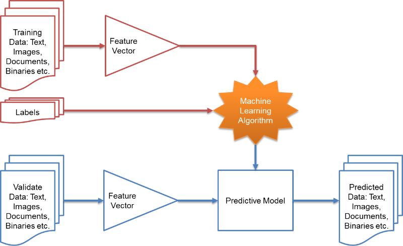 Machine learning can be explained in two ways,
- Machine learning is to find a ‘function’ which describes data the best (by deciding the function parameter).
- Machine learning is to find a ‘probability density’ which describes data the best (by deciding the probability density function parameter).
- e.g. If data was described on gaussian distribution, we have to find the best mean and covariance for the data.
Random Variable
- A random variable is a variable that can take on different values randomly and a description of the states that are possible.
- It must be coupled with a probability distribution that specifies how likely each of these states are.
- Random variables can be discrete or continuous.
Probability Distributions
- Probability distribution is a description of how likely a set of random variables is to take on each of its possible states.
Discrete Variables and PMF
- Probability mass function (PMF) is a probability distribution function over discrete variables.
- PMF maps from a state of a random variable to the probability of that random variable taking on that state.
- Notation: \(P(x = a),\) or \(x \sim P(x)\)
- PMF can act on many variables at the same time which is known as a joint probability distribution.
- \(P(x=a, y=b)\) denotes the probability that \(x=a\) and \(y=b\) simultaneously.
- PMF must satisfy the following properties:
- The domain of \(P\) must be the set of all possible states of \(\tt{x}\).
- \(\forall{x} \in \tt{x}, 0\leq P(x) \leq 1\\) .
- \(\sum_{x\in\tt{x}} P(x) = 1\) (property as being normalized)
Continuous Variables and PDF
- Probability density function (PDF) is a probability distribution function over continuous variables.
- PDF must satisfy the following properties:
- The domain of \(p\) must be the set of all possible states of \(x\).
- \(\forall{x} \in \tt{x}, 0\leq p(x) \leq 1\\) .
- \(\int p(x) dx = 1\) .
- In the univariate example, The probability that \(x\) lies in the interval \([a,b]\) is given by \(\int_{[a,b]}p(x) ds\).
- Uniform distribution on \([a,b]\): \(\tt{x} \sim U(a,b)\)
Marginal Probability
- Marginal probability distribution is a probability distribution over a subset of probability distribution over a set of variables (joint probability distribution).
- For discrete random variables \(\tt{x}\), \(\tt{y}\) and we know \(P(\tt{x}, \tt{y} )\), we can find \(P(\tt{x} )\) with the sum rule:
\[\forall x \in {\tt x}, P({\tt x}= x ) = \sum_y P({\tt x}= x , {\tt y}= y )\]
- For continuous variables, we need to use integration instead of summation:
\[p(x) = \int p(x,y)dy\]
Conditional Probability
- Conditional probability is a probability of some event, given that some other event has happened.
- The conditional probability that \({\tt y} = y\) given \({\tt x} = x\) as \(P({\tt y} = y \mid {\tt x} = x)\) when \(P({\tt x} = x) > 0\)
\[P({\tt y} = y \mid {\tt x} = x) = \frac{P({\tt y} = y, {\tt x} = x)}{P({\tt x} = x)}\]
Chain Rule of Conditional Probabilities
- Chain rule (product rule): Any joint probability distribution over many random variables may be decomposed into conditional distributions over only one variable:
\[P(x^{(1)}, ... , x^{(n)}) = P(x^{(1)})\prod_{i=2}^n P(x^{(i)} \mid x^{(1)}, ... , x^{(i-1)})\\
P(a,b,c) = P(a \mid b,c)P(b,c)\\
P(b,c) = P(b \mid c)P(c)\\
P(a,b,c) = P(a \mid b,c)P(b \mid c)P(c)\]
Independence and Conditional Independence
- Two random variables \({\tt x}\) and \({\tt y}\) are independent (\({\tt x}\perp{\tt y}\)) if their probability distribution can be expressed as a product of two factors, one involving only \({\tt x}\) and one involving only \({\tt y}\):
\[\forall x \in {\tt x}, y \in {\tt y}, p({\tt x} = x, {\tt y} = y)= p({\tt x} = x)p({\tt y} = y)\]
- Two random variables \({\tt x}\) and \({\tt y}\) are conditionally independent (\({\tt x}\perp{\tt y}\mid {\tt z}\)) given a random variable \({\tt z}\) if the conditional probability distribution over \({\tt x}\) and \({\tt y}\) factorizes in this way for every value of \({\tt z}\):
\[\forall x \in {\tt x}, y \in {\tt y}, z \in {\tt z}, p({\tt x} = x, {\tt y} = y \mid {\tt z} = z)= p({\tt x} = x\mid {\tt z} = z)p({\tt y} = y\mid {\tt z} = z)\]
Expectation, Variance and Covariance
Expectation
- Expectation and expected value of some function \(f(x)\) with respect to a probability distribution \(P(x)\) is the average or mean value that \(f\) takes on when \(x\) is drawn from \(P\).
- For discrete variables:
\[E_{x \sim P}[f(x)] = \sum_x P(x)f(x)\]
- For continuous variables:
\[E_{x \sim p}[f(x)] = \int p(x)f(x) dx\]
- Expectations are linear (when \(\alpha\) and \(\beta\) are not dependent on \(x\)):
\[E_x[\alpha f(x) + \beta g(x)] = \alpha E_x[f(x)] + \beta E_x[g(x)]\]
Variance
- Variance gives a measure of how much the values of a function of a random variable \(x\) vary as we sample different values of \(x\) from its probability distribution
\[Var(f(x)) = E[(f(x) - E[f(x)])^2]\]
- When the variance is low, the values of \(f(x)\) cluster near their expected value.
- The square root of the variance is known as the standard deviation.
Covariance
- Covariance gives some sense of how much two values are linearly related to each other, as well as the scale of these variables:
\[Cov(f(x), g(y)) = E[(f(x)-E[f(x)])(g(y)-E[g(y)])]\]
- High absolute values of the covariance mean that the values change very much and are both far from their respective means at the same time.
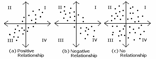
- \(Cov(X,Y) > 0\): \(Y\) increases when \(X\) increases
- \(Cov(X,Y) < 0\): \(Y\) decreases when \(X\) increases
- \(Cov(X,Y) = 0\): there is no linear relation between \(X\) and \(Y\), they are independent, but not always.
- Covariance matrix of a random vector \(x \in R^n\) is an \(n \times n\) matrix, such that
\(Cov(x)_{i,j} = Cov(x_i, X_j)\)
- The diagonal elements of the covariance give the variance: \(Cov(x)_{i,i} = Var(x_i)\)
Correlation
- Correlation normalize the contribution of each variable in order to measure only how much the variables are related, rather than also being affected by the scale of the separate variables.
\[\rho = \frac{Cov(X, Y)}{\sqrt{Var(X)Var(Y)}}, -1\leq\rho\leq1\]
Common Probability Distribution
Bernoulli Distribution
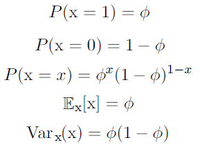
- Bernoulli distribution is a distribution over a single binary random variable.
- It is controlled by a single parameter \(\phi \in [0,1]\), which gives the probability of the random variable being equal to 1.
- It has the following properties:
Multinoulli Distribution
- Multinoulli or categorical distribution is a distribution over a single discrete variable with \(k\) different states, where \(k\) is finite.
- It is parameterized by a vector \(p\in [0,1]^{k-1}\), where \(p_i\) gives the probability of the \(i\)-th state.
- \(k\)-th state’s propability is given by \(1-1^T p\)
- It is often used to refer to distributions over categories of objects.
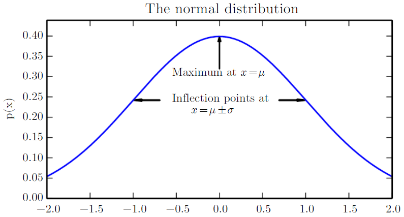
Gaussian Distribution
- Gaussian or normal distribution is the most commonly used distribution over real numbers.
- The mean \(\mu\in R\), the standard deviation \(\sigma\in(0, \infty)\) and the variance by \(\sigma^2\).
\[N(x; \mu, \sigma^2) = \sqrt{\frac{1}{2\pi\sigma^2}}\exp{(-\frac{1}{2\sigma^2})(x-\mu)^2}\]
- When we need to frequently evaluate the PDF, a more efficient way of parametrizing the distribution is to use a parameter \(\beta \in (0,\infty)\) to control the precision or inverse variance of the distribution:
\[N(x; \mu, \beta^{-1}) = \sqrt{\frac{\beta}{2\pi}}\exp{(-\frac{1}{2}\beta)(x-\mu)^2}\]
- The normal distribution generalizes to \(R^n\), in which case it is known as the multivariate normal distribution.
- It is parameterized with a positive definite symmetric matrix \({\bf\Sigma}\).
\[N(x; \mu, {\bf\Sigma}) = \sqrt{\frac{1}{(2\pi)^n\det({\bf\Sigma})}}\exp{(-\frac{1}{2}(x-\mu)^T{\bf\Sigma}^{-1}(x-\mu))}\]
Exponential and Laplace Distributions
- Exponential distribution is often used when we want to have a probability distribution with a sharp point at \(x=0\).
- It uses the indicator function \(1_{x\geq 0}\) to assign probability zero to all negative values of \(x\).
\[p(x;\lambda)=\lambda1_{1\geq 0}\exp(-\lambda x)\]
- A closely related probability distribution that allows us to place a sharp peak of probability mass at an arbitrary point \(\mu\) is the Laplace distribution.
\[Laplace(x;\mu,\gamma)=\frac{1}{2\gamma}\exp(-\frac{\mid x-\mu \mid}{\gamma})\]
Mixtures of Distributions
- Mixtures of Distribution is a distributions made up of several component distributions.
- The choice of which component distribution generates the sample is determined by sampling a component identity from a multinoulli distribution
- \(P(c)\) is the multinoulli distribution over component identities.
\[P(x)=\sum_i P(c=i)P(x\mid c=i)\]
Bayes’ Rule
- When we know \(P(y \mid x)\) and need to know \(P(x \mid y)\), if we also know \(P(x)\) we can compute it using Bayes’ rule.
- \(P(x \mid y)\): posterior which is a probability of the state (event) \(x\) given the data (event) \(y\)
- It is a conditional probability that the likelihood of event \(x\) occurring given that \(y\) is true.
- \(P(y \mid x)\): likelihood which is an observation
- It is a conditional probability that the likelihood of event \(y\) occurring given that \(x\) is true.
- \(P(x)\): prior of \(x\) which is an preliminary information about the state
- It is a marginal probability that the probability of observing \(x\).
- \(P(y)\): prior or evidence of \(y\) which is usually feasible to compute \(P(y) = \sum_x P(y \mid x)P(x)\) or \(P(y) = \int_x P(y \mid x)\).
- It is a marginal probability that the probability of observing \(y\).
- \(P(x \mid y)\): posterior which is a probability of the state (event) \(x\) given the data (event) \(y\)
- Bayes’ Rule where \(x\) and \(y\) are events and \(p(y) \neq 0\):
\[P(x \mid y) = \frac{P(x)P(y \mid x)}{P(y)}\]
Information Theory
Information theory is a branch of applied mathematics that revovles around quantifying how much information is present in a signal.
- In the context of machine learning, a few key ideas from information theory to characterize probability distributions or quantify similarity between probability distributions.
- The basic intuition is that learning that an unlikely event has occurred is more informative than learning that a likely event has occurred.
- Likely events should have low information content, and in the extreme case, events that are guaranteed to happen should have no information content whatsoever.
- Less likely events should have higher information content.
- Independent events should have additive information.
Self-information
- Self-information of an event \({\tt x} =x\):
- Using natural logarithm \(\log\) with base \(e\)
- \(I(x)\) is written in units of nats.
- Self-information deals only with a single outcome.
\[I(x) = -\log P(x)\]
Shannon entropy
- Shannon entropy: Quantify the amount of uncertainty in an entire probability distribution:
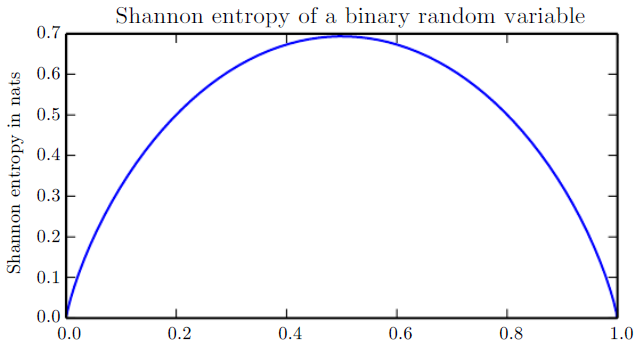
- Shannon entropy of a distribution is the expected amount of information in an event drawn from that distribution.
- Distributions that are nearly deterministic have low entropy, distribution that are closer to uniform have high entropy as shown in the figure.
- When x is continuous, the Shannon entropy is known as the differential entropy.
\[H(x) = E_{x \sim P} [I(x)] = - E_{x \sim P} [logI(x)]\]
Kullback-Leibler (KL) divergence
- If we have two separate probability distributions \(P(x)\) and \(Q(x)\) over the same random variable \(x\), we can measure how different these two distributions are using the KL divergence:
\[D_{KL}(P\parallel Q) = E_{x\sim P}\left[ \log\frac{P(x)}{Q(x)} \right]= E_{x\sim P}[\log P(x) - \log Q(x)]\]
- KL divergence useful properties
- It is non-negative
- KL divergence is 0 if and only if \(P\) and \(Q\) are the same distribution in the case of discrete variables, or equal “almost everywhere” in the case of continuous variables.
- It is often conceptualized as measuring some sort of distance between two distributions.
- However, it is not a true distance measure because it is not symmetric: \(D_{KL}(P\parallel Q) \neq D_{KL}(Q\parallel P)\).
Cross-entropy
- A quantity that is closely related to the KL divergence is the cross-entropy.
\[H(P,Q) = H(P) + D_{KL}(P\parallel Q)= -E_{x\sim P} \log Q(x)\]
- Minimizing the cross-entropy with respect to \(Q\) is equivalent to minimizing the KL divergence, because \(Q\) does not participate in the omitted term.
- \(0\log 0\) is treated as \(\lim_{x\rightarrow0}x\log x = 0\)
Maximum Likelihood Estimation (MLE)
- Maximum Likelihood Estimation (MLE) is a way of parameter estimation or random variable with given observation or data.
- e.g. Imagine if we want to predict \(p\) by throwing a coin with the probability of \(p\) of front and \(1-p\) of back. To compute \(p\) with MLE, we can just divide the number of fronts by the total number of times.
- Consider a set of \(n\) examples \(X = (x_1, x_2, x_3, \ldots, x_n)\) drawn independently from the true but unknown data generating distribution \(f(x)\).
- Let \(p_{model}(x;\theta)\) be a parametric family of probability distributions over the same space indexed by \(\theta\)
- The likelihood can be defined as,
\[\mathcal L (x_1, x_2, \ldots, x_n;\theta) = \mathcal L (X;\theta) = p_{model}(X;\theta) = p_{model}(x_1, x_2, \ldots, x_n;\theta)\]
- MLE \(\theta_{ML}\) which is to maximize the likelihood can be defined as,
\[\theta_{ML} = \arg\max_\theta \mathcal L (X;\theta) = \arg\max_\theta p_{model}(X;\theta) = \arg\max_\theta \prod_{i=1}^m p_{model}(x^{(i)};\theta)\]
-
“In what value of unknown parameter \(\theta\), does the observed data \(X\) get the highest probability?”
-
This product over many probabilities can cause inconvenience such as numerical underflow.
- So, take the logarithm of the likelihood and transform a product into a sum
\[\theta_{ML} = \arg\max_\theta \sum_{i=1}^m \log p_{model}(x^{(i)};\theta)\]
- MLE has a drawback that it is too sensitive to given observation or data.
- e.g. If we throw a coin \(n\) number of time and got \(n\) number of front, MLE can consider it is a coin with only front.
MLE Usage
\[\theta_{ML} = \arg\max_\theta p_{model}(X;\theta)\]- Neural Network
- In training NN, we usually minimize the negative log-likelihood (cross-entropy) which is equivalent to MLE.
- The only constraint to use the negative log-likelihood is to have an output lyaer that can be interpreted as a probability distribution, which we usually we softmax.
- MLE applied to deep networks is called Backpropagation.
- To choose the optimal values of \(\theta\), we use gradient descent where we continually update \(\theta\) in a way that leads to a step up with respect to likelihood.
- Regularization terms can be added and sometimes can be interpreted as prior distributions over the parameters, in that case we are looking for the maximum a posteriori (MAP).
- In training NN, we usually minimize the negative log-likelihood (cross-entropy) which is equivalent to MLE.
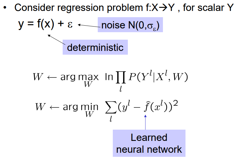 Figure: MLE training for neural networks.
- Linear, logistic regression and multiclass logistic regression
- Conditional random field (CRF)
- Hidden Markov Model (HMM)
Maximum a Posteriori Estimation (MAP)
- Maximum a posteriori estimation (MAP) estimate parameter which has the maximum probability given data, instead of maximizing the probability of data given parameter (MLE).
- MAP estimate chooses the point of maximal posterior probability or maximal probability density in the more common case of continuous \(\theta\).
- As we can only observe \(p(x \mid \theta)\) (likelihood), we use Bayes’ Theroem to use \(p(\theta \mid x)\).
\[\theta_{MAP} = \arg\max_\theta p(\theta \mid x) = \arg\max_\theta log p(x \mid \theta) + \log p(\theta)\]
- MAP Bayesian inference has the advantage of leveraging information that is brought by the prior and connot be found in the training data.
- This additional information helps to reduce the variance in the MAP point estimate compared to the MLE.
- MLE vs. MAP
- Assume we train a logistic regression model,
- MLE training: pick \(W\) to maximize \(P(Y \mid X, W)\)
- MLE training: pick \(W\) to maximize \(P(W \mid X, Y)\)
- If a prior information is given as part of the problem, then use MAP.
- If not, we cannot use MAP and MLE is a reasonable approach.
- Assume we train a logistic regression model,
MAP Usage
- Neural Network
- MAP is closely related to the method of MLE, but employs an augmented optimization objective which incorporates a prior distribution over the quantity one want to estimate.
- MAP estimation can therefore be seen as a regularization of MLE.
 Figure: MAP training for neural networks.
- Bayesian Neural Network
- Hidden Markov Model (HMM)