Learn the basics about Convolutional Neural Network (CNN), its detail and case models of CNN.
Comparison Between CNN and FFNN
In the figure below, left is a regular 3-layer neural network and right is a CNN arranges its neurons in three dimensions (width, height, depth). The red input layer in CNN holds the image, so its width and height would be the dimensions of the image, and the depth would be 3 (Red, Green, Blue channels).
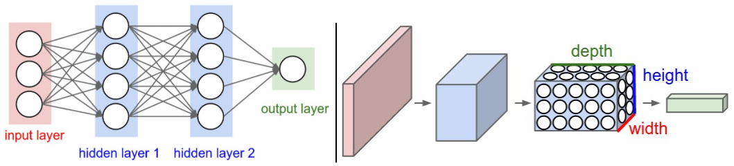
- Regular neural network do not scale well to full images
- Fully-connected structure does not scale to larger image. (e.g. \(200 \times 200 \times 3\) would lead to neurons that have 120,000 weights).
- 3D volumes of neurons
- CNN have neurons arranged in 3 dimensions: width, height, depth (depth: third dimension of an activation volume).
- The neurons in a layer will only be connected to a small region of the layer, instead of all of the neurons in a fully-connected manner.
- CNN will reduce the full image into a single vector of class scores, arranged along the depth dimension.
Convolution
Naive Convolution
- Time Complexity
- When the image size \(N\) and filter size \(a\)
- Time complexity of 1D convolution will be \(O(aN) \approx O(N^2)\).
- When the image size \(N \times N\) and filter size \(a \times b\)
- Time complexity of 2D convolution will be \(O(abN^2) \approx O(N^4)\).
- When the image size \(N \times N \times N\) and filter size \(a \times b \times c\)
- Time complexity of 3D convolution will be \(O(abcN^3) \approx O(N^6)\).
- When the image size \(N\) and filter size \(a\)
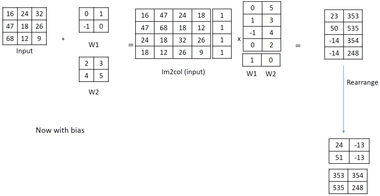
Convolution by Matrix Computation
By using matrix computation, the convolution computation can be done faster than the naive way. It can be done by using a doubly block circulant matrix which is a special case of Toeplitz matrix.
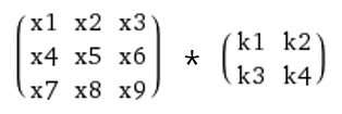
When you have 2d input \(x\) with size \(n \times n\) and 2d kernel \(k\) with size \(m \times m\), and you want to calculate the convolution \(x*k\), you can unroll \(k\) into a sparse matrix of size \((n-m+1)^2 \times n^2\) and unroll \(x\) into a long vector \(x^2 \times 1\). You compute a multiplication of the sparse matrix with a vector and convert the resulting vector with size \((n-m+1)^2 \times 1\) into a \(n-m+1\) square matrix.
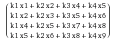
For example,
The constructed matrix with a vector will be,
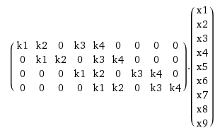
which will be equal to,
The result is equal to convolution by doing a sliding window of \(k\) over \(x\).
The other way around is possible as well, for example,
- Time Complexity
- When the image size \(N \times N\) and filter size \(a \times b\), Time complexity of 2D convolution will be \(O(N^3)\).
Convolution by Fast Fourier Transform (FFT)
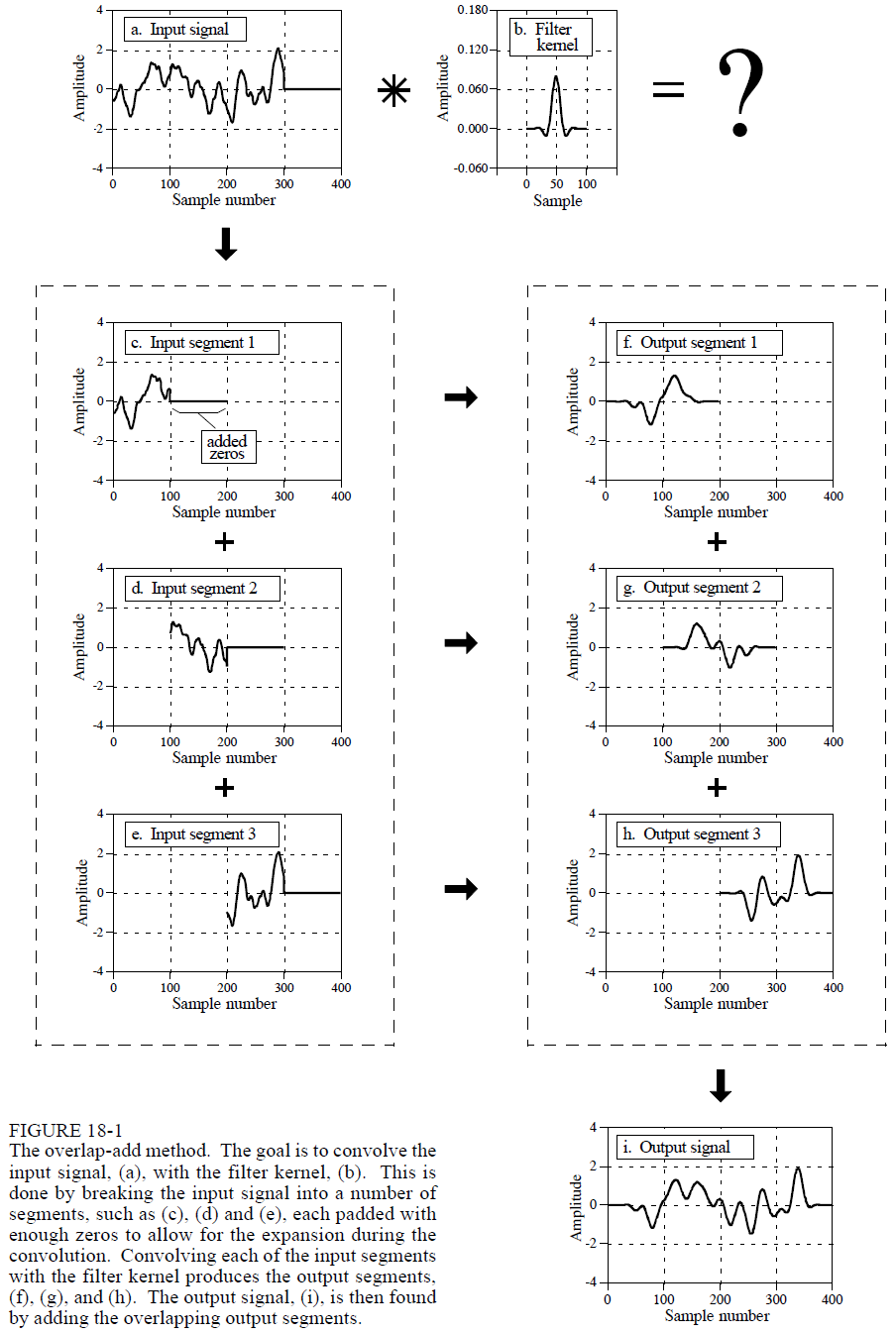
By using Fast Fourier Transform (FFT), the convolution computation can be done faster. FFT convolution uses the principle that multiplication in the frequency domain corresponds to convolution in the time domain. The input signal is transformed into the frequency domain using the DFT, multiplied by the frequency response of the filter, and then transformed back into the time domain using the Inverse DFT. FFT convolution uses the overlap-add method shown in below figure.
- Time Complexity
- When the image size \(N\) and filter size \(a\)
- Time complexity of 1D convolution will be \(O(N \log N)\).
- When the image size \(N \times N\) and filter size \(a \times b\)
- Time complexity of 2D convolution will be \(O(N^2 \log_2 N)\).
- When the image size \(N \times N \times N\) and filter size \(a \times b \times c\)
- Time complexity of 3D convolution will be \(O(N^3 \log_3 N)\).
- When the image size \(N\) and filter size \(a\)
CNN Layers
Convolutional neural network usually use three main types of layers: Convolutional Layer, Pooling Layer, Fully-Connected Layer.
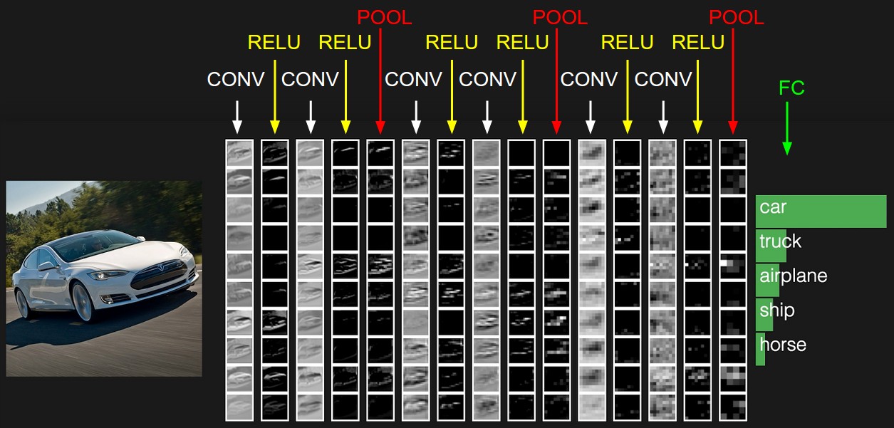
- Example architecture for overview: a simple CNN for CIFAR-10 classification could have the architecture [INPUT - CONV - RELU - POOL - FC]
- INPUT [32x32x3] will hold the raw pixel values of the image, in this case an image of width 32, height 32, and with three color channels R,G,B.
- CONV layer will compute the output of neurons that are connected to local regions in the input, each computing a dot product between their weights and a small region they are connected to the input volume. This may result in volume such as [32x32x12] if we decided to use 12 filters.
- RELU layer will apply an element-wise activation function, such as the \(max(0,x)\) thresholding at zero. This leaves the size of the volume unchanged [32x32x12].
- POOL layer will perform a downsampling operation along the spatial dimensions (width, height), resulting in volume such as [16x16x12].
- FC layer will compute the class scores, resulting in volume of size [1x1x10], where each of the 10 numbers correspond to a class score as of CIFAR-10.
- Notes
- Each layer may or may not have parameters (e.g. CONV/FC do, RELU/POOL don’t)
- These parameters will be traned with gradient descent so that the class scores that the ConvNet computes are consistent with the labels in the training set for each image.
- Each layer may or may not have additional hyperparameters (e.g. CONV/FC/POOL do, RELU doesn’t)
- Below figure is an example activations of CNN where the initial volume stores the raw image pixels and the last volume stores the class scores.
- Each layer may or may not have parameters (e.g. CONV/FC do, RELU/POOL don’t)
Convolutional Layer
- Local Connectivity
- CNN connect each neuron to only a local region of the input volume as It is impractical to connect neurons to all neurons in the previous volume for high-dimensional inputs such as images.
- The spatial extent of this connectivity is a hyperparameter called the receptive field of the neuron (equivalently to filter size).
- The extent of the connectivity along the depth axis is always equal to the depth of the input volume.
- An example is shown in below figure where each neuron is connected only to a local region with full depth (i.e. all color channels) and there are multiple neurons (5 in this example) all looking the same region in the input.
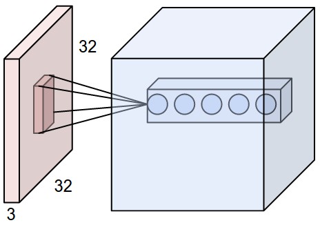
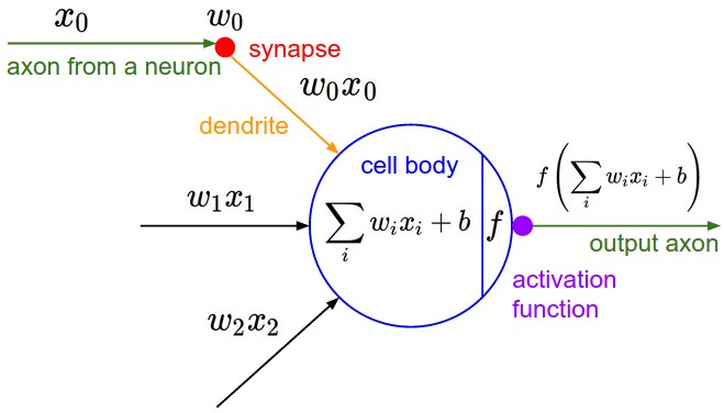
- As shown in below figure, the neurons still compute a dot product of their weights with the input followed by a non-linearity (same with FFNN), but their connectivity is now restricted to be local spatially.
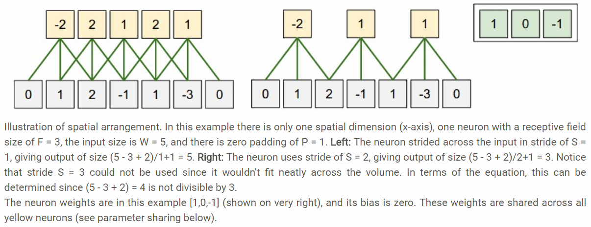
- Spatial Arrangement
- Three hyperparameters control the size of the output volume: the depth, stride and zero-padding.
- Depth: It corresponds to the number of filters, each learning to look for something different in the input such as, presence of various oriented edges, or blobs of color.
- Refer to a set of neurons that are all looking at the same region of the input as a depth column
- Stride: it is for sliding the filter, when the stride is 2 then the filters jump 2 pixels at a time.
- Zero-padding: Sometimes it will be convenient to pad the input volume with zeros around the border.
- It allows us to control the spatial size of the output volumes.
- Formula to compute the spatial size of the output volume: \((W-F+2P)/S+1\)
- where input volume size (W), the receptive field size (F), the stride (S), the amount of zero padding (P)
Pooling Layer
- What is pooling layer?
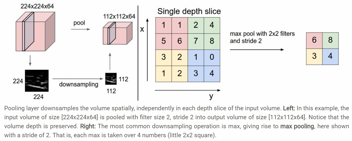
- Pooling layer is to progressively reduce the spatial size of the representation to reduce the amount of parameters and computation in the network, and hence to also control overfitting.
- It operates independently on every depth slice of the input and resizes it spatially, using the MAX operation.
- The most common form is with fiters of size 2x2 applied with a stride of 2 downsamples every depth slice.
- The depth dimension remains unchanged.
- Pooling layer
- Accepts a volume of size \(W_1 \times H_1 \times D_1\)
- Requires two hyperparameters: their spatial extent \(F\), the stride \(S\)
- Produces a volume of size \(W_2 \times H_2 \times D_2\) where:
- \[W_2 = (W_1 - F) / S + 1\]
- \[H_2 = (H_1 - F) / S + 1\]
- \[D_2 = D_1\]
- Introduces zero parameters since it computes a fixed function of the input
- It is not common to use zero-padding for pooling layers
- General pooling
- Only two commonly seen variations of the max pooling layer found in practice:
- A pooling layer with \(F=3, S=2\) (called overlapping pooling)
- A pooling layer with \(F=2, S=2\)
- Pooling sizes with larger receptive fields are too destructive.
- There are other functions, such as average pooling and L2-norm pooling. But they has fallen out of favor compared to the max pooling.
- Only two commonly seen variations of the max pooling layer found in practice:
- Getting rid of pooling
- Discarding pooling layers has also been found to be important in training good generative models, such as variational autoencoders (VAEs) or generative adversarial networks(GANs).
Fully-Connected Layer
- Neurons in a fully connected layer have full connections to all activations in the previous layer.
- Their activations can hence be computed with a matrix multiplication followed by a bias offset.
- This layer work as a classification purpose.
Softmax Loss
Cross-entropy loss with softmax function as below figure is one of the most common used supervision components in CNNs. The softmax loss is defined in this paper as the combination of a cross-entropy loss, a softmax function and the last fully connected layer. It has been used widely because of its simplicity and clear probabilistic interpretation. Despite its popularity, the paper have shown that it has limitation of the lack of encouraging the discriminability of CNN features.
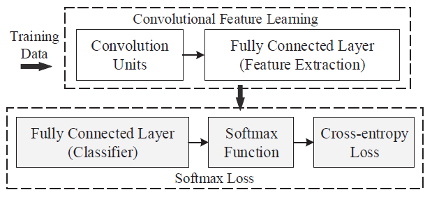 Figure: Cross-entropy loss together with softmax function is one of the most common used supervision components in CNN
Several CNN Models
- LeNet: The first successful applications of CNN were developed in 1990’s.
- AlexNet: The first work that popularized CNN in Computer Vision.
- The network had a very similar architecture to LeNet, but was deeper, bigger, and feature Convolutional Layers stacked on top of each other
- Previously it was common to only have a single CONV layer always immediately followed by a POOL layer)
- ZF Net: It was an improvement on AlexNet by tweaking the architecture hyperparameters
- In particular by expanding the size of the middle convolutional layers and making the stride and filter size on the first layer smaller.
- GoogLeNet: Its main contribution was the development of an Inception Module that dramatically reduced the number of parameters in the network (4M, compared to AlexNet with 60M).
- Additionally, this paper uses Average Pooling instead of Fully Connected layers at the top of the ConvNet, eliminating a large amount of parameters that do not seem to matter much.
- Thare are also several followup versions to the GoogLeNet, most recently Inception-v4.
- VGGNet: Its main contribution was in showing that the depth of the network is a critical component for good performance.
- Their final best network contains 16 CONV/FC layers and features an extremely homogeneous architecture that only performs 3x3 convolutions and 2x2 pooling from the beginning to the end.
- A downside of the VGGNet is that it is more expensive to evaluate and uses a lot more memory and parameters (140M).
- Most of these parameters are in the first fully connected layer, and it was since found that these FC layers can be removed with no performance downgrade, significantly reducing the number of necessary parameters.
- ResNet: Residual Network features special skip connections and a heavy use of batch normalization.
- The architecture is also missing fully connected layers at the end of the network.
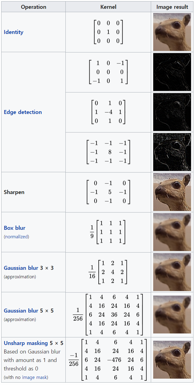
Famous Convolution Fiter
- Depending on the element values (convolution filters), a kernel can cause a wide range of effects.