‘Batch Normalization’ is an basic idea of a neural network model which was recorded the state-of-the art (4.82% top-5 test error) in the ImageNet competition ILSVRC2015. It was published and presented in International Conference on Machine Learning (ICML) 2015 with a paper name ‘Batch Normalization: accelerating Deep Network Training by Reducing Internal Covariate Shirt’.
Introduction
Summary
- Problem Statement
- Internal Covariate Shift: Distribution of each layer’s inputs changes during training, as the parameters of the previous layers change.
- This slows down the training by requiring lower learning rates and careful parameter initialization.
- Research Objective
- To address the internal covariate shift problem and accelerate the training of deep neural nets.
- Solution Proposed: Batch Normalization
- Batch normalization takes a step towards reducing internal covariate shift, and in doing so dramatically accelerates the training of deep neural nets.
- It accomplishes this via a normalization step that fixes the means and variances of each layer input in training mini-batch.
- Contribution
- Batch normalization allows to use much higher learning rates, less careful about initialization and works as regularization (no need for dropout).
Motivation
- Stochastic gradient descent (SGD) is a widely used gradient method using mini-batch for training a deep neural network.
- Pros
- The gradient of the loss over a mini-batch is an estimate of the gradient over the training set, whose quality improves as the batch size increases.
- The computation over a mini-batch can be more efficient than computations for individual examples on modern computing platforms.
- Cons
- This requires careful tuning of the learning rate, and the initial parameter values.
- One naive way to increase training speed is to increase the learning rate, but high learning rate usually leads to gradient vanishing or gradient exploding.
- Pros
- Internal Covariate Shift: Distribution of each layer’s inputs changes during training, as the parameters of the previous layers change.
- Small changes to the network parameters amplify as the network becomes deeper.
- The saturation problem and the resulting vanishing gradients are usually addressed by using ReLU, careful initialization, and small learning rate.
- If we could ensure that the distribution of nonlinearity inputs remains more stable as the network trains, then the optimizer would be less likely to get stuck in the saturated regime, and the training would accelerate.
Reducing Internal Covariate Shift with Whitening
- Whitening: One naive approach to reduce internal covariate shift by normalizing the input distribution into normal distribution with zero mean and unit variance (LeCun 1998, Wiesler & Ney 2011).
- With a given column data \(X\in R^{d\times n}\), whitening transform is,
\[\hat{X} = Cov(X)^{-1/2} X \\
Cov(X) = E[( X - E[X] ) ( X - E[X] )^\top ]\]
- Drawbacks of whitening approach
- It requires high computation since it needs to compute \(Cov(X)^{-1/2}\) for normalizing multi variate normal distribution.
- It needs more computation to decide mean and variance of all data in each training step.
Batch Normalization Transform
Two Simplifications
Since the full whitening of each layer’s inputs is costly, we make two simplifications.
- First simplification: we will normalize each scalar feature independently, by making it have zero mean and unit variance.
- For a layer with \(d\)-dimentional input \(x = (x^{(1)}, x^{(2)}, \ldots, x^{(d)})\), we will normalize each dimension,
\[\hat{x}^{(k)} = \frac{x^{(k)} - E[x^{(k)}]}{\sqrt{Var[x^{(k)}]}}.\]
- Simply normalizing each input of a layer may change what the layer can represent.
- e.g. normalizing the inputs of a sigmoid would constrain them to the linear regime of the non-linearity.
- To address this, we make sure that the transformation inserted in the network can represent the identity transform.
- For each activation \(x^(k)\), a pair of parameters \(\gamma, \beta\), which scale and shift the normalized value and are learned along with the original model parameters,
\[y^{(k)} = \gamma \hat{x}^{(k)} + \beta.\]
- Second simplification: Since we use mini-batches in stochastic gradient training, each mini-batch produces estimates of the mean and variance of each activation instead of those of full-batch.
- This way, the statistics used for normalization can fully participate in the gradient backpropagation.
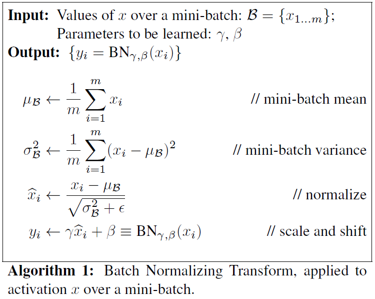
Batch Normalizing Transform
- Refer to the transform \(BN_{\gamma, \beta} : x_{1...m} \rightarrow y_{1...m}\) as the Batch Normalizing Transform.
- When \(\epsilon\) is a constant added to the mini-batch variance for numerical stability.
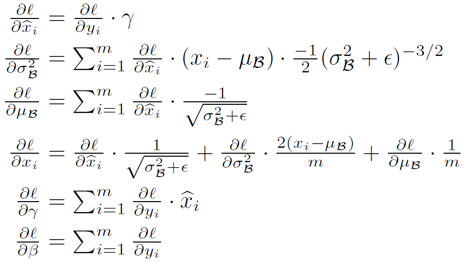
- Chain rule for batch normalizing transform
Training and Inference
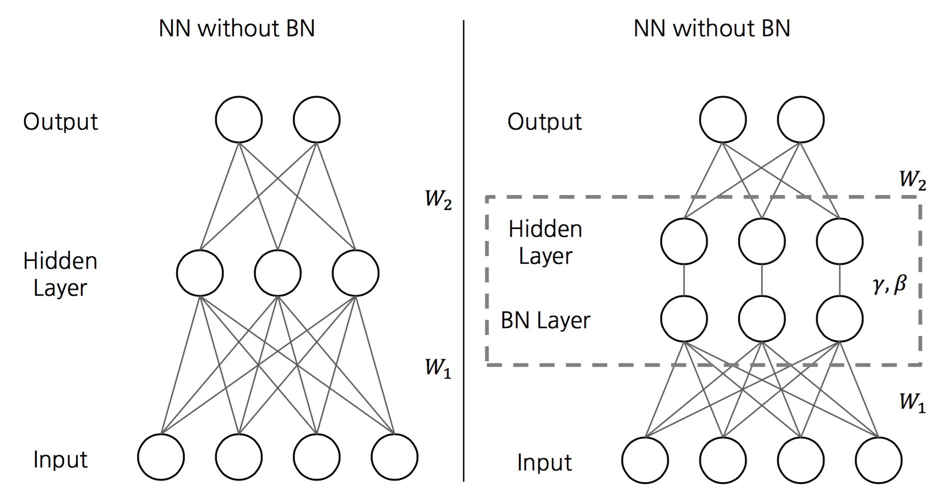
- To Batch-normalize a network, we specify a subset of activations and insert the BN transform for each of them.
- Specifically, after computing \(wx+b\) and before computing activation function of each layer.
- Specifically, after computing \(wx+b\) and before computing activation function of each layer.
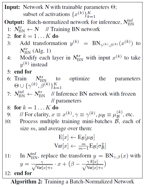
- The procedure for training batch-normalized networks.
- Train the network by using BN transform with the sample mean and variance of mini-batch.
- The normalization of activations that depends on the mini-batch allows efficient training, but is neither necessary nor desirable during inference.
- We want the output to depend only on the input, deterministically.
- Test the network by using BN transform with unbiased mean and variance estimator which are computed with saved sample mean and variance.
- Train the network by using BN transform with the sample mean and variance of mini-batch.
Contributions of BN
- BN networks can be trained with saturating nonlinearities
- It prevents small changes in layer parameters from amplifying as the data propagates through a deep network.
- e.g. It helps the sigmoid nonlinearities to more easily stay in their non-saturated regimes
- More tolerant to increased training rates (higher learning rate)
- Reduce internal covariate shift, more resilient to the parameter scale
- Faster convergence
-
Less careful initialization
- Regularization effect (Dropout is unnecessary)
- To amplify the effect of regularization, decide the mini-batch by shuffling the training data.
Experiments
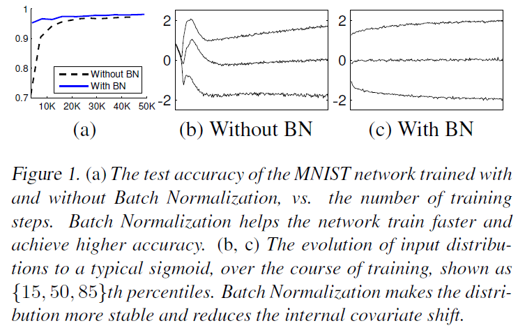
Activations Over Time
- Figure 1(a) shows faster convergence and higher test accuracy of BN network.
- Figure 1(b) and (c) plot the activation value while training, and BN network have similar distribution from the beginning to the end.
ImageNet Classification
-
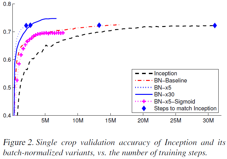
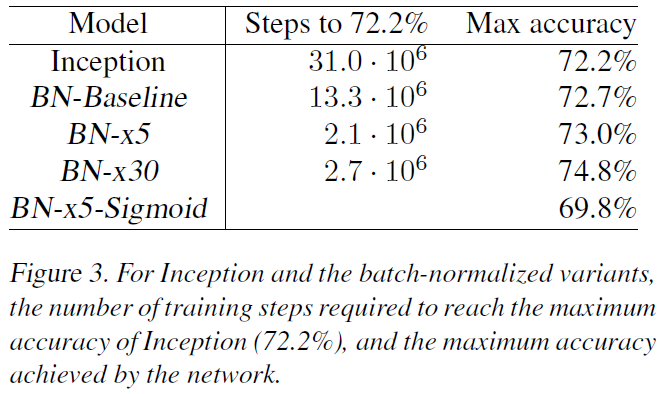
Figure 2 and 3 compares Inception network by varying the learning rate, and BN network gives faster convergence and higher max accuracy.
-
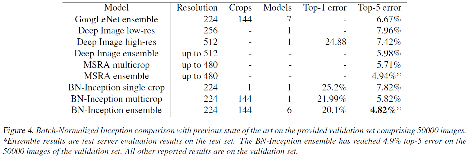
BN network achieves the state-of-the-art on ImageNet competition with small parameter tunning
Accelerating BN Nets
- Increase learning rate: faster convergence
- Remove Dropout: BN works as regularization
- Shuffle training examples more thoroughly: to get different model for generalization
- Reduce the \(L_2\) weight regularization: BN works as regularization
- Accelerate the learning rate decay: BN nets trains faster
- Remove Local Response Normalization: not suitable for BN
- Reduce the photometric distoritions: because BN nets train faster and observe each training example fewer times, it is better to focus on more “real” images
References
- Paper: Batch Normalization: Accelerating Deep Network Training by Reducing Internal Covariate Shift [Link]