This post will be about artificial intelligence related terms including linear algebra, probability distribution, machine learning and deep learning
B
Bootstrapping
- Bootstrapping is any test or metric that relies on random sampling with replacement.
- It allows assigning measures of accuracy to sample estimates.
- Bootstrapping is the practice of estimating properties of an estimator by measuring those properties when sampling from an approximating distribution.
- Bootstrapping sample is a random sample conducted with replacement.
- Steps:
- Randomly select an observation from the original data.
- “Write it down”
- “Put it back” (i.e. any observation can be selected more than once)
- Repeat steps 1-3 \(N\) times: \(N\) is the number of observations in the original sample.
- Steps:
- Reference
Blob Detection
In computer vision, *blob detection methods are aimed at detecting regions in a digital image that differ in properties, such as brightness or color, compared to surrounding regions. Informally, a blob is a region of an image in which some properties are constant or approximately constant; all the points in a blob can be considered in some sense to be similar to each other. The most common method for blob detection is convolution.
- Reference
- Wikipedia: Blob detection
C
Collaborative Filtering
- Collaborative filtering (CF) is a technique used by recommender system and it has two sense, a narrow one and a general one.
- In the narrow sense, collaborative filtering is a method of making automatic predictions (filtering) about the interests of a user by collecting preferences or taste information from many users (collaborating).
- In the more general sense, collaborative filtering is the process of filtering for information or patterns using techniques involving collaboration among multiple agents, viewpoints, data sources, etc.
- CF based on users’ past behavior have two categories:
- User-based: measure the similarity between target users and other users
- Item-based: measure the similarity between the items that target users rates/interacts with and other items
-
The key idea behind CF is that similar users share the same interest and that similar items are liked by a user.
- Reference
D
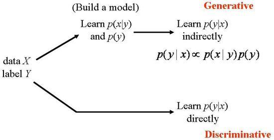
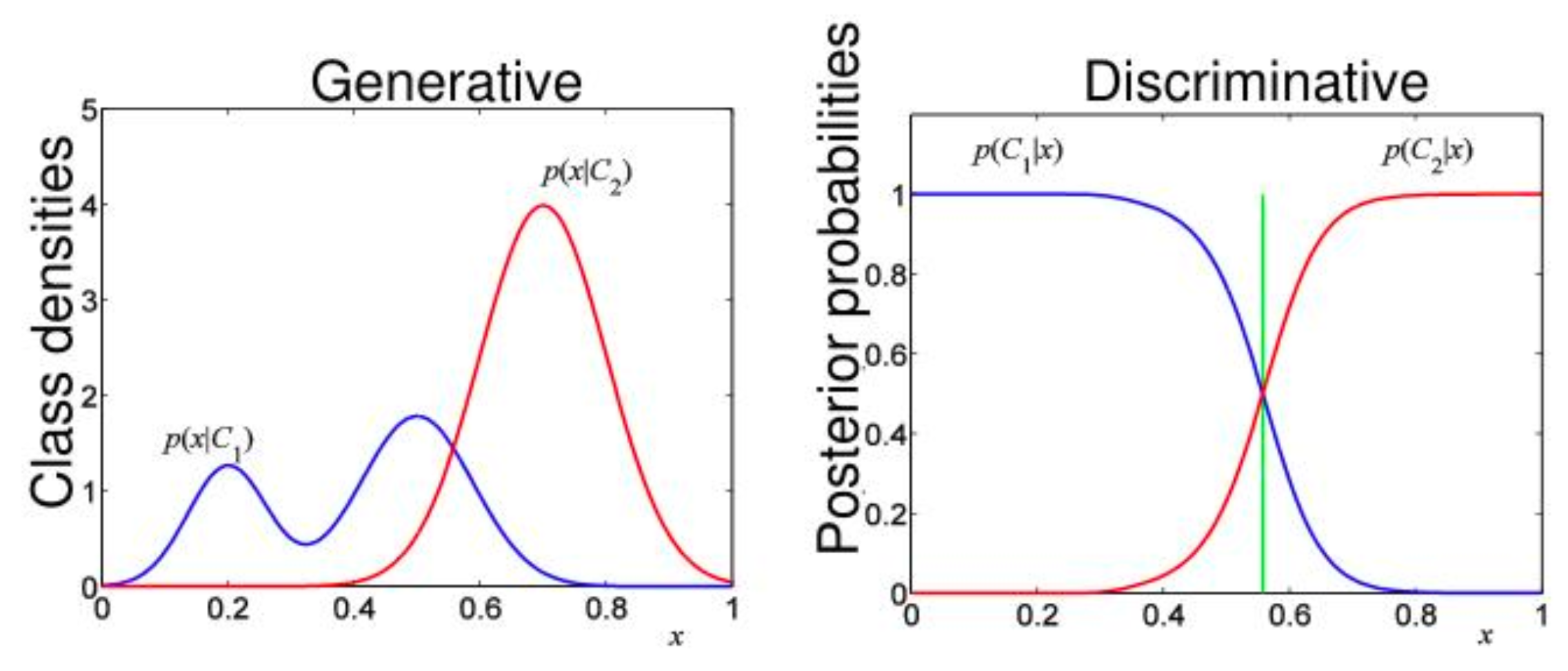
Discriminative Model
- Discriminative model directly estimate class probability (posterior probability) \(p(y \mid x)\) given input
- Some methods do not have probabilistic interpretation, but fit a function \(f(x)\), and assign to classes based on it
- Focus on the decision boundary
- More powerful with lots of examples
- Not designed to use unlabeled data
- Only supervised tasks
-
Examples: Gaussians, Naive-Bayesian, Mixtures of multinomial, Mixtures of Gaussians, Hidden Markov Models, Bayesian Networks, Morkov Random Fields
-
Check the generative model for comparison
-
Reference
Deterministic Model
- Deterministic model is a mathematical model in which outcomes are precisely determined through known relationships among states and events, without room for random variation.
- A deterministic model always performs the same way for a given set of same initial conditions.
- It hypothesized an exact relationship between variables which allows one to make predictions and see how one variable affects the other.
-
Example: (Deterministic) Neural Network, (Deterministic) Regression model
-
Check the probabilistic model for comparison
- Reference
G
Generative Model
- Generative model compute of posterior probability \(p(y \mid x)\) using bayes rule to infer distribution over class given input
- Model the density of inputs \(x\) from each class \(p(x \mid y)\)
- Estimate class prior probability \(p(y)\)
- Probabilistic model of each class
- Natural use of unlabeled data
-
Examples: Logistic Regression, Gaussian Process, Regularization Networks, Support Vector Machines, Neural Networks
-
Check the discriminative model for comparison
-
Reference
Graphical Model
H
Hamming Distance
In information theory, the Hamming distance between two strings of equal length is the number of positions at which the corresponding symbols are different. In other words, it measures the minimum number of substitutions required to change one string into the other, or the minimum number of errors that could have transformed one string into the other. In a more general context, the Hamming distance is one of several string metrics for measuring the edit distance between two sequences.
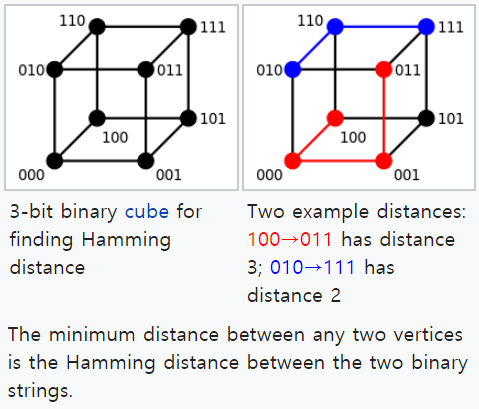 Figure : Example of hamming distance.
- Reference
- Wikipedia: Hamming distance
Hard Negative Mining
- Hard positive cases: anchor and positive samples that are far apart
- Hard negative cases: anchor and negative samples that are close together
-Hard-mining strategies: Bootstrapping offers a lot of liberties on how the hard examples are chosen. One could for instance pick a limited number of false positives per image or one could fix a threshold and only pick a false positive if its score is superior to a fixed threshold (0.5 for instance).
- Hard negative class mining: greadily selects negative classes in a relatively efficient manner, as opposed to negative “instance” mining. It is executed as follows:
- Evaluate embedding vectors: choose randomly a large number of output classes C; for each class, randomly pass a few (one or two) examples to extract their embedding vectors.
- Select negative classes: select one class randomly from C classes from step 1. Next, greedily add a new class that violates triplet constraint the most w.r.t. the selected classes till we reach N classes. When a tie appears, we randomly pick one of tied classes.
- Finalize N-pair: draw two examples from each selected class from step 2.
- Reference
I
Image Localization, Detection, Segmentation
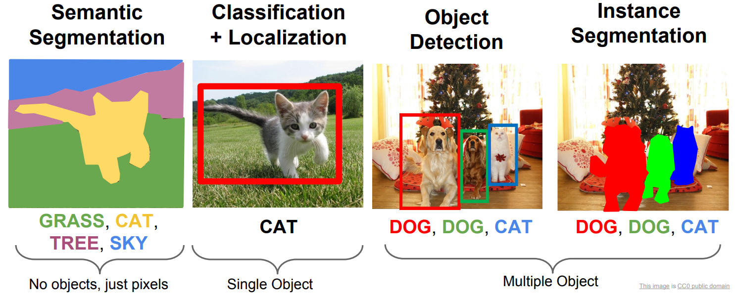
- Reference
- Slide: Stanford CS231 [Link]
Invariance vs. Equivariance
Invariance to a transformation means if you take the input and transform it then the representation you get the same as the representation of the original, i.e. represent(x) = represent(transform(x))
Equivariance to a transformation means if you take the input and transform it then the representation you get is a transformation of the representation of the original, i.e. transform(represent(x)) = represent(transform(x)).
Replicated feature detectors are equivariant with respect to translation, which means that if you translate the input then the representation you get is a translation of the representation of the original.
- Reference
L
Latent Variable
-
Latent variables are variables that are not directly observed but are rather inferred from other variables that are observed (directly measured).
-
Reference
- Wikipedia: Latent variable [Link]
Latent Variable Model
- Latent variable model is a statistical model that relates a set of observable variables to a set of latent variables.
- It aims to explain observed variables in terms of latent variables.
- Reference
- Wikipedia: Latent variable model [Link]
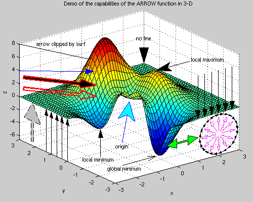
Local Minimum Problem
- Local minimum problem happens when the backpropagation network converge into a local minima instead of the desired global minimum since the error value is very complex function with many parameter values of weights.
- The backpropagation algorithm employs gradient descent by following the slope of error value downward along with the change in all the weight values.
- The weight values are constantly adjusted until the error value is no longer decreasing.
- Local minimum problem can be avoided with several solutions
- Utilize momentum which gradually increases the weight adjustment rate
- Use stochastic gradient descent is more likely to jump out of a local minimum and find a global minimum, but still can get stuck in local minimum.
- In stochastic gradient descent, the parameters are estimated for every observation (mini-batch), as opposed the whole sample (full-batch) in regular gradient descent.
- This gives lots of randomness and the path of stochastic gradient descent wanders over more places.
- Adding noise to the weights while being updated
-
Check the saddle point for comparison
- Reference
- ECE Edu: Local Minimum problem [Link]
M
Metric Learning
Metric Learning is the task of learning a distance function over objects. A metric or distance function has to obey four axioms: non-negativity, Identity of indiscernibles, symmetry and subadditivity / triangle inequality. In practice, metric learning algorithms ignore the condition of identity of indiscernibles and learn a pseudo-metric.
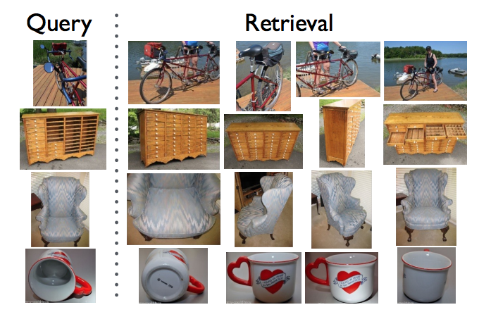 Figure: Example of metric learning application
- Reference
- Wikipedia: Similarity learning
Mean Squared Error
Mean squared error(MSE) or mean squared deviation (MSD) of an estimator measures the average of the squares of the errors or deviations. The MSE is a measure of the quality of an estimator which is always non-negative, and values closer to zero are better.
- Predictor
- If \(\hat{Y}\) is a vector of \(n\) predictions, and \(Y\) is the vector of observed values of the variable being predicted
- The MSE is the mean \(\left(\frac{1}{n}\sum_{i=1}^n \right)\) of the squares of the errors (\((Y_i-\hat{Y_i})^2\))
- Estimator
- The MSE of an estimator \(\hat{\theta}\) with respect to an unknown parameter \(\theta\) is defined as
- Reference
- Wikipedia: Mean squared error [Link]
Multiple Instance Learning (MIL)
Multiple instance learning (MIL) is a variation on supervised learning. Instead of receiving a set of instances which are individually labeled, the learner receives a set of labeled bags, each containing many instances.
Given an image, we want to know its target class based on its visual content. For instance, the target might be “beach”, where the image contains both “sand” and “water” In MIL terms, the image is described as a bag \(X={X_1, \cdots, X_N}\), where each \(X_i\) is the feature vector (called instance) extracted from the corresponding \(i\)-th region in the image and \(N\) is the total regions (instances) partitioning the image. The bag is labeled positive (“beach”) if it contains both “sand” region instances and “water” region instances.
- Reference
- Wikipedia: Multiple-instance learning [Link]
O
Object Proposal
Object proposal is a hypothesis that is proposed which is not yet a successful detection but just a proposal that needs to be verified and refined.
-
It can be wrong but the trick is to reduce the chances of object detection being wrong.
-
Reference
- Quora: What’s the difference between object detection and object proposals? [Link]
P
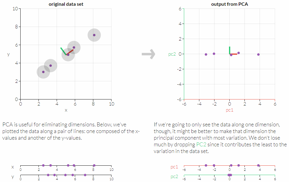
Principal Component Analysis (PCA)
Principal component analysis (PCA) is a dimension-reduction tool that can be used to reduce a large set of variables to a small set that still contains most of the information in the large set.
- PCA is a mathematical procedure that transforms a number of (possibly) correlated variables into a (smaller) number of uncorrelated variables called principal components.
- Reference
Probabilistic Model
- Probabilistic (stochastic) model is a mathematical representation of a random phenomenon which is defined by its sample space, events within the sample space, and probabilities.
- Unlike the deterministic model, the probabilistic model includes elements of randomness.
- This model is likely to produce different results even with the same initial conditions.
- There is always an element of chance or uncertainty involved which implies that there are possible alternate solutions.
-
Example: (Probabilistic) Regression models, Probability tress, Monte Carlo, Markov models, Stochastic Neural Network
-
Check the deterministic model for comparison
- Reference
R
RIP vs. ROP
-
Rotation-In-Plane (RIP): Rotation within a plane in two dimensional space
-
Rotation-Off-Plane (ROP): Spatial rotation in three dimensional space
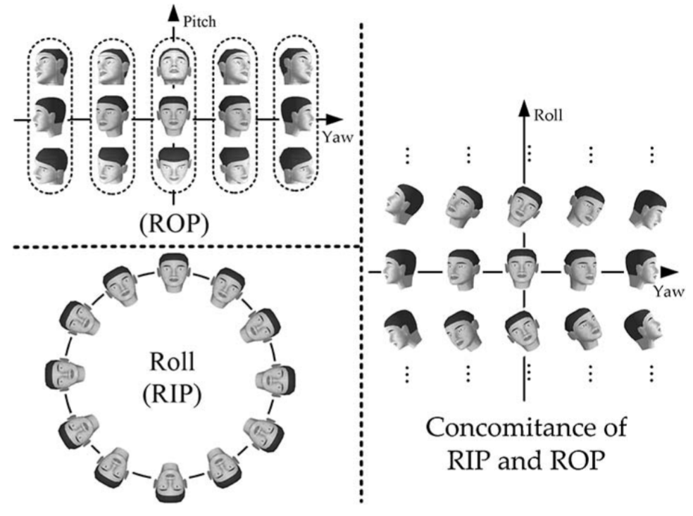 Figure: Faces of RIP, ROP, respectively, and concomitance of both RIP and ROP.
- Reference
S
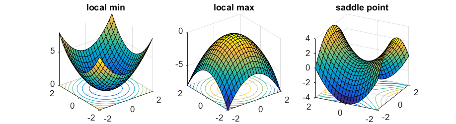
Saddle Point
- Saddle point is a point on the surface of a function where the slopes (derivatives) of orthogonal function components defining the surface become zero but are not a local extremum on both axes.
- The critical point with a relative minimum along one axial direction and at a relative maximum along the other axial direction.
- When we optimize neural networks, for most of the trajectory we optimize, the critical points (the points where the derivative is zero or close to zero) are saddle points.
- Saddle points, unlike local minima, are easily escapable
-
Check the local minimum problem for comparison
-
Reference
- Wikipedia: Saddle point [Link]
Sparse Data
- Sparse data is data that is easily compressed.
- Depending on the type of data that you’re working with, it usually involves empty slots where data would go.
- Matrices, for instance, that are have lots of zeroes can be compressed and take up significantly less space in memory.
- Reference
- Web: Data Modeling - What means “Data is dense/sparse” ? [Link]
W
Weakly Supervised Learning
- Weakly supervised learning is a term covering a variety of studies that attempt to construct predictive models by learning with weak supervision (incomplete, inexact and inaccurate supervision).
- It can be supervision with noisy labels. (e.g. bootstrapping, where the bootstrapping procedure may mislabel some examples)
- Three types of weak supervision
- Incomplete supervision: where only a subset of training data is given with labels
- Inexact supervision: where the training data are given with only coarse-grained labels
- Inaccurate supervision: where the given labels are not always ground-truth
- Bootstrapping is one of weakly supervised learning method, which is also called self-training, it is a form of learning that is designed to use less training examples.
- It starts with a few training examples, trains a classifier, and uses thought-to-be positive examples as yielded by this classifier for retraining.
- As the set of training examples grow, the classifier improves, provided that not too many negative examples are misclassified as positive, which could lead to deterioration of performance.
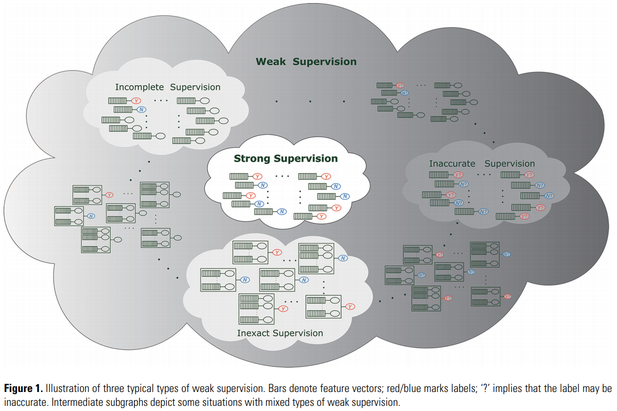
 Figure: Hierarchy tree of supervision.