“Super-Convergence: very fast training of neural networks using large learning rates” suggests a different learning rate policy called ‘one cycle policy’ which makes network to be trained significantly faster and named this phenomenon ‘super-convergence’.
Summary
- Research Objective
- This paper describe a phenomenon, which named “super-convergence”, where neural networks can be trained an order of magnitude faster than with standard training methods.
- Proposed Solution
- One of the key elements of super-convergence is training with one learning rate cycle and a large maximum learning rate.
- Contribution
- Systematically investigates a new training methodology with improved speed and performance.
- Demonstrates that large learning rates regularize training and other forms of regularization must be reduced to maintain an optimal balance of regularization.
- Derives a simplification of the second order, Hessian-free optimization method to estimate optimal learning rates which demonstrates that large learning rates find wide, flat minima.
- Demonstrates that the effects of super-convergence are increasingly dramatic when less labeled training data is available.
Cyclical Learning Rates
The idea of Super-convergence is based on the previous research of the author: Cyclical learning rates for training neural networks.
Problem Statement
- It is known that the learning rate is the most important hyper-parameter to tune for training deep neural networks.
- It is well known that too small a learning rate will make a training algorithm converge slowly while too large a learning rate will make the training algorithm diverge.
- Hence, one must experiment with a variety of learning rates and schedules, which can be troublesome work.
Research Objective
- To eliminates the need to experimentally find the best values and schedule for the global learning rates.
Proposed Solution
- Cyclical learning rates: instead of monotonically decreasing the learning rate, this method lets the learning rate cyclically vary between reasonable boundary values.
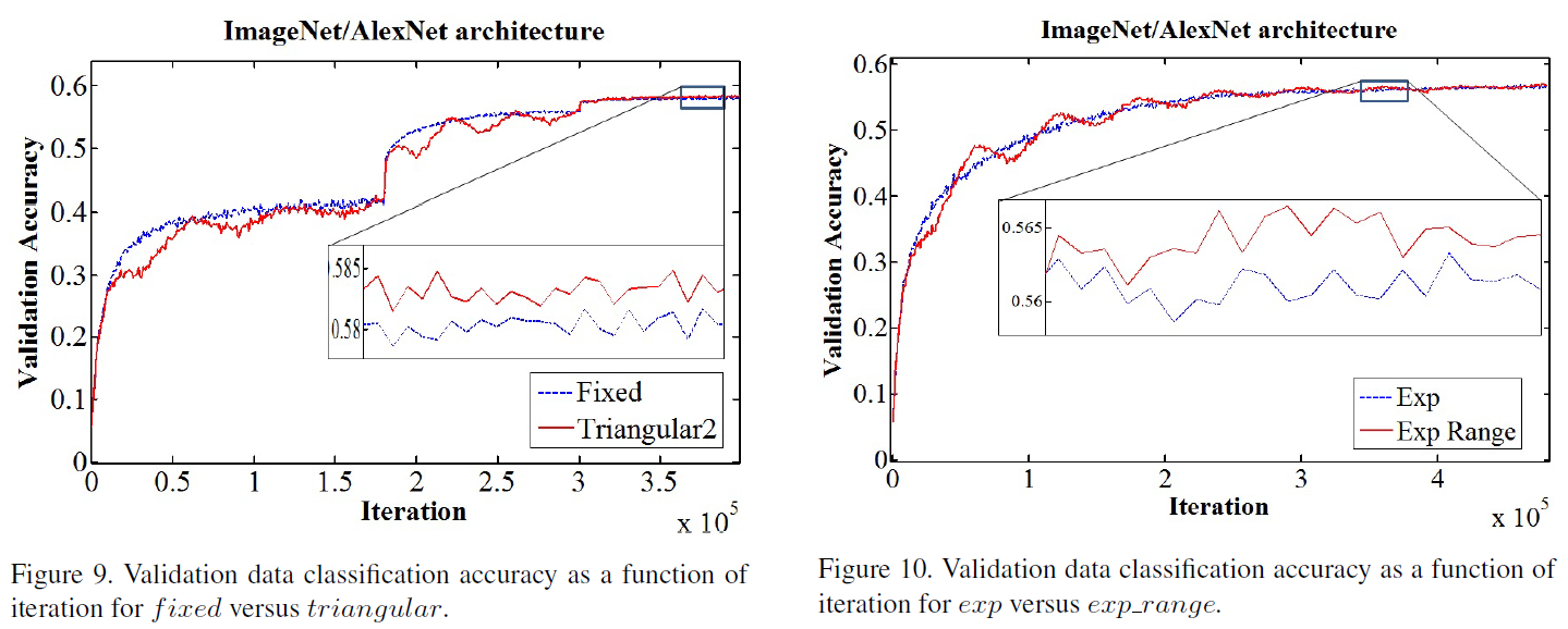
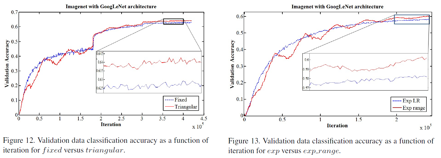
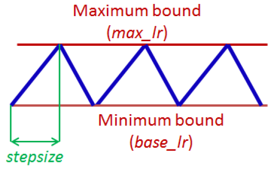 Figure 1: Triangular learning rate policy. The blue lines represent learning rate values changing between bounds. The input parameter stepsize is the number of iterations in half a cycle.
- How can one estimate a good value for the cycle length?
- The final accuracy results are actually quite robust to cycle length but experiments show that it often is good to set stepsize equal to 2 - 10 times the number of iterations in an epoch.
- How can one estimate reasonable minimum and maximum boundary values?
- “LR range test”: run your model for several epochs while letting the learning rate increase linearly between low and high LR values.
- And find reasonable minimum and maximum boundary values with one training run of the network for a few epochs.
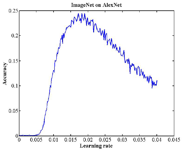 Figure 2: AlexNet LR range test; validation classification accuracy as a function of increasing learning rate. base lr = 0.006 and max lr = 0.014.
Contribution
- Training with cyclical learning rates instead of fixed values achieves improved classification accuracy without a need to tune and often in fewer iterations.
- This paper also dexcribes a simple way to estimate “reasonable bounds” - linearly increasing the learning rate of the network for a few epochs.
Super-convergence
- In this work, super-convergence use cyclical learning rates (CLR) and the learning rate range test (LR range test).
- The LR range test can be used to determine if super-convergence is possible for an architecture.
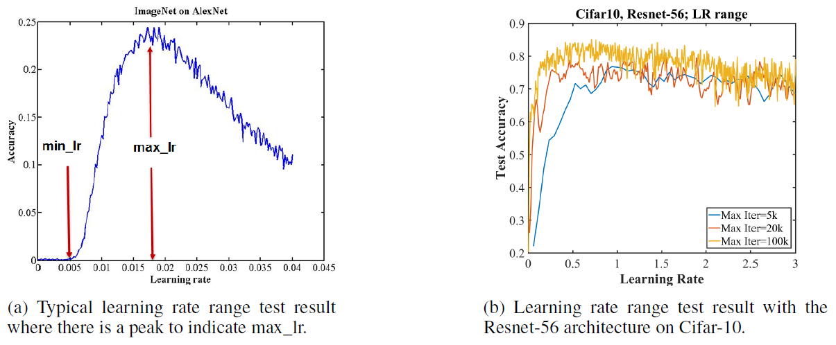
Figure 3: Comparison of learning rate range test results.
- Fig 3-a. shows typical curve from a LR range test, where the test accuracy has a distinct peak.
- The learning rate at this peak is the largest value to use as the maximum learning rate bound when using CLR
- The minimum learning rate can be chosen by dividing the maximum by a factor of 3 or 4.
- Fig 3-b. shows that the test accuracy remains consistently high over this unusual range of large learning rates.
- This unusual behavior is indicative of potential for super-convergence.
- 1 Cycle: slight modification of cyclical learning rate policy for super-convergence
- Always use one cycle that is smaller than the total number of iterations/epochs
- And allow the learning rate to decrease several orders of magnitude less than the initial learning rate for the remaining iterations.
- The general principle of regularization: The amount of regularization must be balanced for each dataset and architecture
- Recognition of this principle permits general use of super-convergence.
- Reducing other forms of regularization and regularizing with very large learning rates makes training significantly more efficient.
Optimizer
- Investigation whether adaptive learning rate methods in a piecewise constant training regime would learn to adaptively use large learning rates to improve training speed and performance.
- Tested Nesterov momentum, AdaDelta, AdaGrad, Adam on Cifar-10 with the Resnet-56.
- None of these methods speed up the training process in a similar fashion to super-convergence.
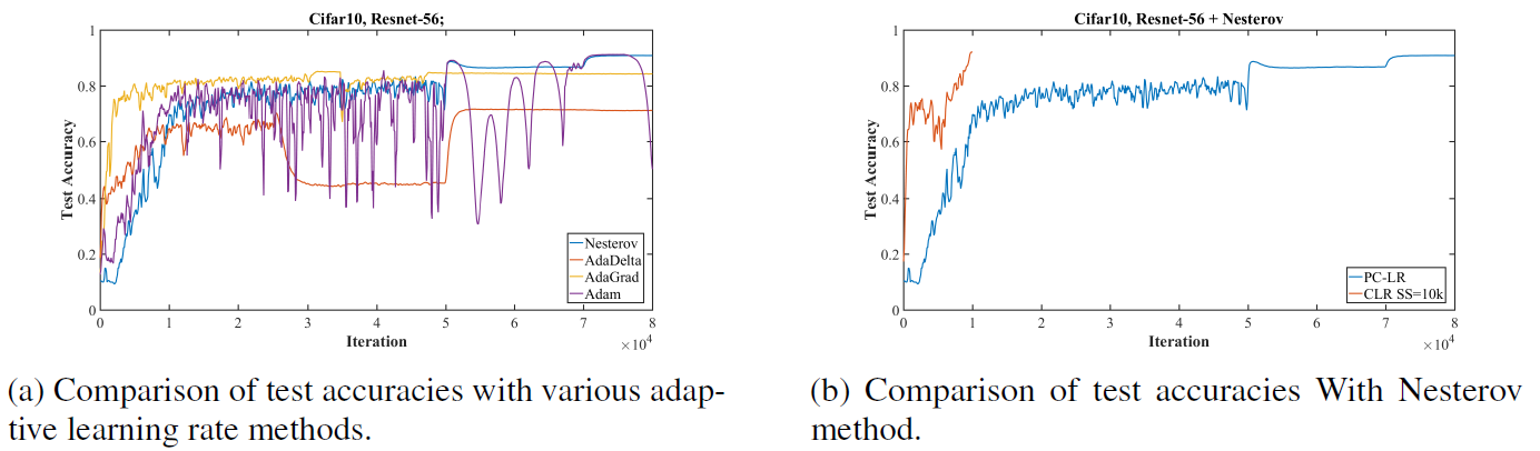
Figure 4: Comparisons for Cifar-10, Resnet-56 of super-convergence to piecewise constant training regime.
- Investigation whether adaptive learning methods with the 1cycle learning rate policy can bring super-convergence phenomenon.
- Nesterov, AdaDelta, and AdaGrad allowed super-convergence to occur.
Estimating Optimal Learning Rates
- This paper derives a simplification of the second order, Hessian-free optimization method to estimate optimal learning rates.
- It is not feasible to compute the Hessian matrix because of computation matter.
- Hessian expresses the curvature in all directions in a high dimensional space, but the only relevant curvature direction is in the direction of steepest descent that SGD will traverse.
- This concept is contained within Hessian-free optimization.
- The AdaSecant method builds an adaptive learning rate method by it and we can calculate optimal learning rate for each of the neurons.
- This paper suggests the way of estimating of the global learning rate from the weight specific rates by summing over the numerator and denominator.
- The large learning rates indicated by these Figures is caused by small values of Hessian approximation and small values of the Hessian implies that SGD is finding flat and wide local minima.
In this paper we do not perform a full evaluation of the effectiveness of this technique as it is tangential to the theme of this work. We only use this method here to demonstrate that training with large learning rates are indicated by this approximation. We leave a full assessment and tests of this method to estimate optimal adaptive learning rates as future work.
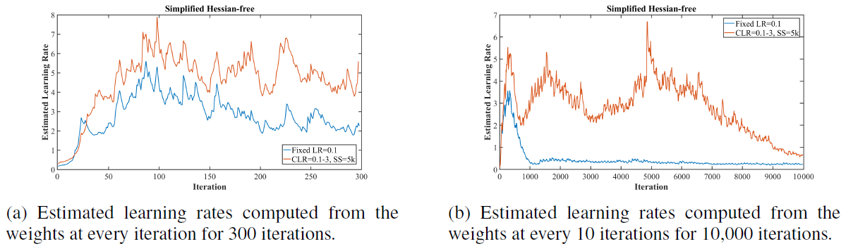
Figure 5: Estimated learning rate from the simplified Hessian-free optimization while training. The computed optimal learning rates are in the range from 2 to 6.
Experiments
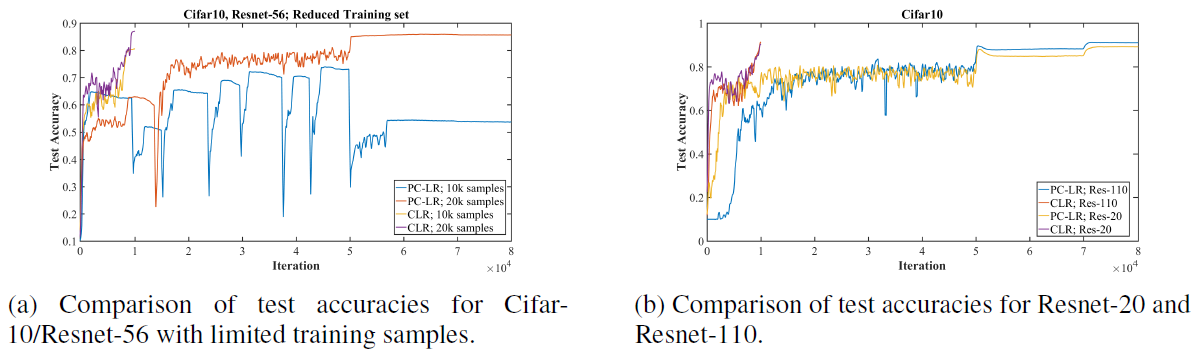
Figure 6: Comparisons of super-convergence to typical training outcome with piecewise constant learning rate schedule.
- Fig 6-a provides a comparison of super-convergence with a reduced number of training samples.
- When the amount of training data is limited, the gap in performance between the result of standard training and super-convergence increases.
- Fig 6-b illustrates the results for Resnet-20 and Resnet-110.
- Resnet-20: CLR 90.4% vs. PC-LR: 88.6%, Resnet-110: CLR: 92.1% vs. PC-LR 91.0%
- The accuracy increase due to super-convergence is greater for the shallower architectures.
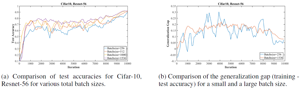
Figure 7: Comparisons of super-convergence to over a range of batch sizes. These results show that a large batch size is more effective than a small batch size for super-convergence training.
- Fig 7 shows experiments on the effects of larger batch size and the generalization gap (the difference between the training and test accuracies).
- In Fig 7-a, super-convergence training gives improvement in performance with larger batch sizes.
- In Fig 7-b, it shows that the generalization gap are approximately equivalent for small and large mini-batch sizes.
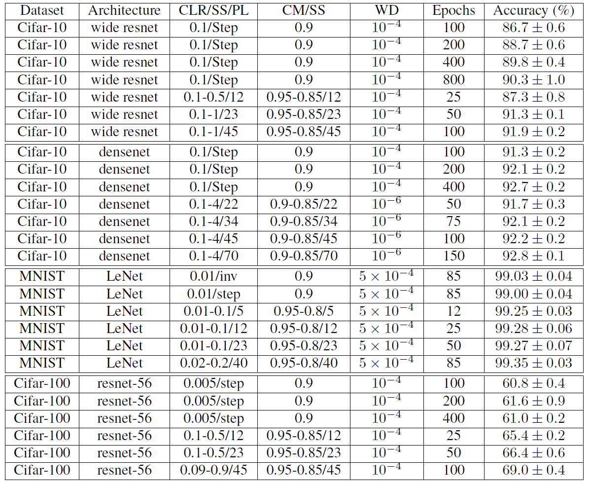
Figure 8: Final accuracy and standard deviation for various datasets and architectures. The total batch size (TBS) for all of the reported runs was 512. PL = learning rate policy or SS = stepsize in epochs, where two steps are in a cycle, WD = weight decay, CM = cyclical momentum. Either SS or PL is provide in the Table and SS implies the cycle learning rate policy.
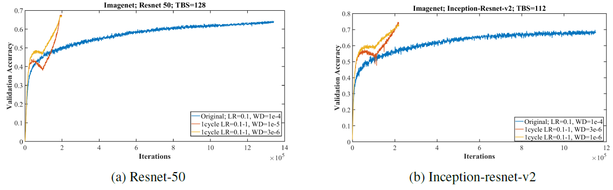
Figure 9: Training resnet and inception architectures on the imagenet dataset with the standard learning rate policy (blue curve) versus a 1cycle policy that displays super-convergence. Illustrates that deep neural networks can be trained much faster (20 versus 100 epochs) than by using the standard training methods.
- In the Fig 9, experiments with Imagenet show that reducing regularization in the form of weight decay allows the use of larger learning rates and produces much faster convergence and higher final accuracies.
- The learning rate varying from 0.05 to 1.0, then down to 0.00005 in 20 epochs.
- In order to use such large learning rates, it was necessary to reduce the value for weight decay.