Probability

Learn about probability which are the basics of artificial intelligence and deep learning.

Probability

Two Perspectives of Machine Learning

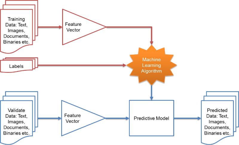Machine learning can be explained in two ways,

1. Machine learning is to find a ‘function’ which describes data the best (by deciding the function parameter).
2. Machine learning is to find a ‘probability density’ which describes data the best (by deciding the probability density function parameter).
   • e.g. If data was described on gaussian distribution, we have to find the best mean and covariance for the data.

Random Variable

• A random variable is a variable that can take on different values randomly and a description of the states that are possible.
  • It must be coupled with a probability distribution that specifies how likely each of these states are.
  • Random variables can be discrete or continuous.

Probability Distributions

• Probability distribution is a description of how likely a set of random variables is to take on each of its possible states.

Discrete Variables and PMF

• Probability mass function (PMF) is a probability distribution function over discrete variables.
  • PMF maps from a state of a random variable to the probability of that random variable taking on that state.
  • Notation: \(P(x = a),\) or \(x \sim P(x)\)
• PMF can act on many variables at the same time which is known as a joint probability distribution.
  • \(P(x=a, y=b)\) denotes the probability that \(x=a\) and \(y=b\) simultaneously.
• PMF must satisfy the following properties:
  • The domain of \(P\) must be the set of all possible states of \(\tt{x}\).
  • \(\forall{x} \in \tt{x}, 0\leq P(x) \leq 1\\) .
  • \(\sum_{x\in\tt{x}} P(x) = 1\) (property as being normalized)

Continuous Variables and PDF

• Probability density function (PDF) is a probability distribution function over continuous variables.
• PDF must satisfy the following properties:
  • The domain of \(p\) must be the set of all possible states of \(x\).
  • \(\forall{x} \in \tt{x}, 0\leq p(x) \leq 1\\) .
  • \(\int p(x) dx = 1\) .
• In the univariate example, The probability that \(x\) lies in the interval \([a,b]\) is given by \(\int_{[a,b]}p(x) ds\).
  • Uniform distribution on \([a,b]\): \(\tt{x} \sim U(a,b)\)

Marginal Probability

• Marginal probability distribution is a probability distribution over a subset of probability distribution over a set of variables (joint probability distribution).
• For discrete random variables \(\tt{x}\), \(\tt{y}\) and we know \(P(\tt{x}, \tt{y} )\), we can find \(P(\tt{x} )\) with the sum rule:

\[\forall x \in {\tt x}, P({\tt x}= x ) = \sum_y P({\tt x}= x , {\tt y}= y )\]

• For continuous variables, we need to use integration instead of summation:

\[p(x) = \int p(x,y)dy\]

Conditional Probability

• Conditional probability is a probability of some event, given that some other event has happened.
• The conditional probability that \({\tt y} = y\) given \({\tt x} = x\) as \(P({\tt y} = y \mid {\tt x} = x)\) when \(P({\tt x} = x) > 0\)

\[P({\tt y} = y \mid {\tt x} = x) = \frac{P({\tt y} = y, {\tt x} = x)}{P({\tt x} = x)}\]

Chain Rule of Conditional Probabilities

• Chain rule (product rule): Any joint probability distribution over many random variables may be decomposed into conditional distributions over only one variable:

\[P(x^{(1)}, ... , x^{(n)}) = P(x^{(1)})\prod_{i=2}^n P(x^{(i)} \mid x^{(1)}, ... , x^{(i-1)})\\ P(a,b,c) = P(a \mid b,c)P(b,c)\\ P(b,c) = P(b \mid c)P(c)\\ P(a,b,c) = P(a \mid b,c)P(b \mid c)P(c)\]

Independence and Conditional Independence

• Two random variables \({\tt x}\) and \({\tt y}\) are independent (\({\tt x}\perp{\tt y}\)) if their probability distribution can be expressed as a product of two factors, one involving only \({\tt x}\) and one involving only \({\tt y}\):

\[\forall x \in {\tt x}, y \in {\tt y}, p({\tt x} = x, {\tt y} = y)= p({\tt x} = x)p({\tt y} = y)\]

• Two random variables \({\tt x}\) and \({\tt y}\) are conditionally independent (\({\tt x}\perp{\tt y}\mid {\tt z}\)) given a random variable \({\tt z}\) if the conditional probability distribution over \({\tt x}\) and \({\tt y}\) factorizes in this way for every value of \({\tt z}\):

\[\forall x \in {\tt x}, y \in {\tt y}, z \in {\tt z}, p({\tt x} = x, {\tt y} = y \mid {\tt z} = z)= p({\tt x} = x\mid {\tt z} = z)p({\tt y} = y\mid {\tt z} = z)\]

Expectation, Variance and Covariance

Expectation

• Expectation and expected value of some function \(f(x)\) with respect to a probability distribution \(P(x)\) is the average or mean value that \(f\) takes on when \(x\) is drawn from \(P\).
• For discrete variables:

\[E_{x \sim P}[f(x)] = \sum_x P(x)f(x)\]

• For continuous variables:

\[E_{x \sim p}[f(x)] = \int p(x)f(x) dx\]

• Expectations are linear (when \(\alpha\) and \(\beta\) are not dependent on \(x\)):

\[E_x[\alpha f(x) + \beta g(x)] = \alpha E_x[f(x)] + \beta E_x[g(x)]\]

Variance

• Variance gives a measure of how much the values of a function of a random variable \(x\) vary as we sample different values of \(x\) from its probability distribution

\[Var(f(x)) = E[(f(x) - E[f(x)])^2]\]

• When the variance is low, the values of \(f(x)\) cluster near their expected value.
• The square root of the variance is known as the standard deviation.

Covariance

• Covariance gives some sense of how much two values are linearly related to each other, as well as the scale of these variables:

\[Cov(f(x), g(y)) = E[(f(x)-E[f(x)])(g(y)-E[g(y)])]\]

• High absolute values of the covariance mean that the values change very much and are both far from their respective means at the same time.
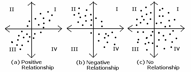
  • \(Cov(X,Y) > 0\): \(Y\) increases when \(X\) increases
  • \(Cov(X,Y) < 0\): \(Y\) decreases when \(X\) increases
  • \(Cov(X,Y) = 0\): there is no linear relation between \(X\) and \(Y\), they are independent, but not always.
• Covariance matrix of a random vector \(x \in R^n\) is an \(n \times n\) matrix, such that \(Cov(x)_{i,j} = Cov(x_i, X_j)\)
  • The diagonal elements of the covariance give the variance: \(Cov(x)_{i,i} = Var(x_i)\)

Correlation

• Correlation normalize the contribution of each variable in order to measure only how much the variables are related, rather than also being affected by the scale of the separate variables.

\[\rho = \frac{Cov(X, Y)}{\sqrt{Var(X)Var(Y)}}, -1\leq\rho\leq1\]

Common Probability Distribution

Bernoulli Distribution

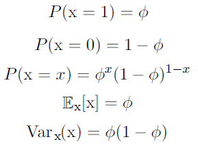
• Bernoulli distribution is a distribution over a single binary random variable.
  • It is controlled by a single parameter \(\phi \in [0,1]\), which gives the probability of the random variable being equal to 1.
  • It has the following properties:

Multinoulli Distribution

• Multinoulli or categorical distribution is a distribution over a single discrete variable with \(k\) different states, where \(k\) is finite.
  • It is parameterized by a vector \(p\in [0,1]^{k-1}\), where \(p_i\) gives the probability of the \(i\)-th state.
  • \(k\)-th state’s propability is given by \(1-1^T p\)
  • It is often used to refer to distributions over categories of objects.

Gaussian Distribution

• Gaussian or normal distribution is the most commonly used distribution over real numbers.
  • The mean \(\mu\in R\), the standard deviation \(\sigma\in(0, \infty)\) and the variance by \(\sigma^2\).

\[N(x; \mu, \sigma^2) = \sqrt{\frac{1}{2\pi\sigma^2}}\exp{(-\frac{1}{2\sigma^2})(x-\mu)^2}\]

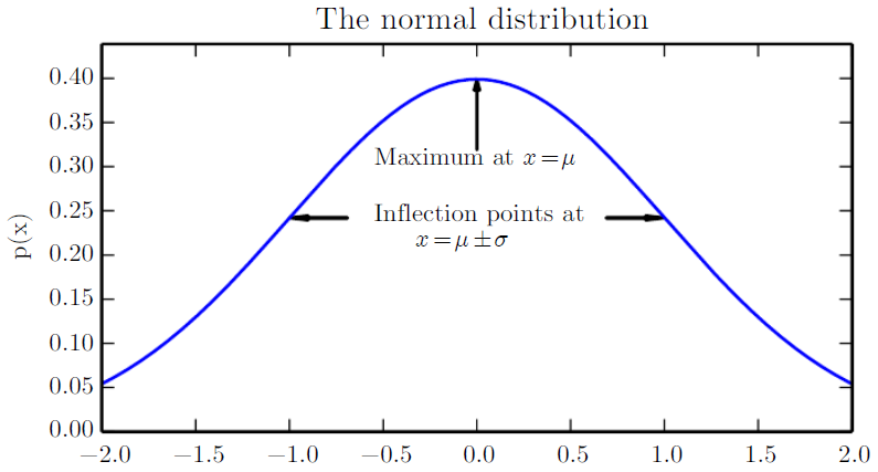
• When we need to frequently evaluate the PDF, a more efficient way of parametrizing the distribution is to use a parameter \(\beta \in (0,\infty)\) to control the precision or inverse variance of the distribution:

\[N(x; \mu, \beta^{-1}) = \sqrt{\frac{\beta}{2\pi}}\exp{(-\frac{1}{2}\beta)(x-\mu)^2}\]

• The normal distribution generalizes to \(R^n\), in which case it is known as the multivariate normal distribution.
  • It is parameterized with a positive definite symmetric matrix \({\bf\Sigma}\).

\[N(x; \mu, {\bf\Sigma}) = \sqrt{\frac{1}{(2\pi)^n\det({\bf\Sigma})}}\exp{(-\frac{1}{2}(x-\mu)^T{\bf\Sigma}^{-1}(x-\mu))}\]

Exponential and Laplace Distributions

• Exponential distribution is often used when we want to have a probability distribution with a sharp point at \(x=0\).
  • It uses the indicator function \(1_{x\geq 0}\) to assign probability zero to all negative values of \(x\).

\[p(x;\lambda)=\lambda1_{1\geq 0}\exp(-\lambda x)\]

• A closely related probability distribution that allows us to place a sharp peak of probability mass at an arbitrary point \(\mu\) is the Laplace distribution.

\[Laplace(x;\mu,\gamma)=\frac{1}{2\gamma}\exp(-\frac{\mid x-\mu \mid}{\gamma})\]

Mixtures of Distributions

• Mixtures of Distribution is a distributions made up of several component distributions.
  • The choice of which component distribution generates the sample is determined by sampling a component identity from a multinoulli distribution
  • \(P(c)\) is the multinoulli distribution over component identities.

\[P(x)=\sum_i P(c=i)P(x\mid c=i)\]

Bayes’ Rule

• When we know \(P(y \mid x)\) and need to know \(P(x \mid y)\), if we also know \(P(x)\) we can compute it using Bayes’ rule.
  • \(P(x \mid y)\): posterior which is a probability of the state (event) \(x\) given the data (event) \(y\)
    • It is a conditional probability that the likelihood of event \(x\) occurring given that \(y\) is true.
  • \(P(y \mid x)\): likelihood which is an observation
    • It is a conditional probability that the likelihood of event \(y\) occurring given that \(x\) is true.
  • \(P(x)\): prior of \(x\) which is an preliminary information about the state
    • It is a marginal probability that the probability of observing \(x\).
  • \(P(y)\): prior or evidence of \(y\) which is usually feasible to compute \(P(y) = \sum_x P(y \mid x)P(x)\) or \(P(y) = \int_x P(y \mid x)\).
    • It is a marginal probability that the probability of observing \(y\).
• Bayes’ Rule where \(x\) and \(y\) are events and \(p(y) \neq 0\):

\[P(x \mid y) = \frac{P(x)P(y \mid x)}{P(y)}\]

Information Theory

Information theory is a branch of applied mathematics that revovles around quantifying how much information is present in a signal.

• In the context of machine learning, a few key ideas from information theory to characterize probability distributions or quantify similarity between probability distributions.
• The basic intuition is that learning that an unlikely event has occurred is more informative than learning that a likely event has occurred.
  • Likely events should have low information content, and in the extreme case, events that are guaranteed to happen should have no information content whatsoever.
  • Less likely events should have higher information content.
  • Independent events should have additive information.

Self-information

• Self-information of an event \({\tt x} =x\):
  • Using natural logarithm \(\log\) with base \(e\)
  • \(I(x)\) is written in units of nats.
  • Self-information deals only with a single outcome.

\[I(x) = -\log P(x)\]

Shannon entropy

• Shannon entropy: Quantify the amount of uncertainty in an entire probability distribution:
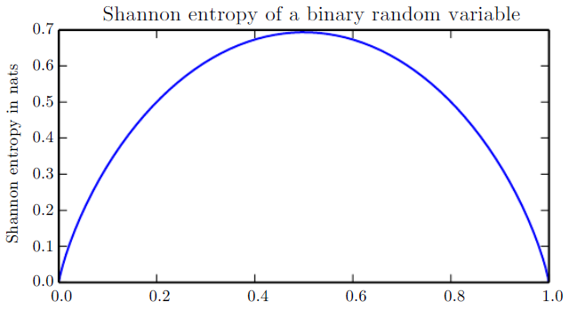
• Shannon entropy of a distribution is the expected amount of information in an event drawn from that distribution.
• Distributions that are nearly deterministic have low entropy, distribution that are closer to uniform have high entropy as shown in the figure.
• When x is continuous, the Shannon entropy is known as the differential entropy.

\[H(x) = E_{x \sim P} [I(x)] = - E_{x \sim P} [logI(x)]\]

Kullback-Leibler (KL) divergence

• If we have two separate probability distributions \(P(x)\) and \(Q(x)\) over the same random variable \(x\), we can measure how different these two distributions are using the KL divergence:

\[D_{KL}(P\parallel Q) = E_{x\sim P}\left[ \log\frac{P(x)}{Q(x)} \right]= E_{x\sim P}[\log P(x) - \log Q(x)]\]

• KL divergence useful properties
  • It is non-negative
  • KL divergence is 0 if and only if \(P\) and \(Q\) are the same distribution in the case of discrete variables, or equal “almost everywhere” in the case of continuous variables.
  • It is often conceptualized as measuring some sort of distance between two distributions.
    • However, it is not a true distance measure because it is not symmetric: \(D_{KL}(P\parallel Q) \neq D_{KL}(Q\parallel P)\).

Cross-entropy

• A quantity that is closely related to the KL divergence is the cross-entropy.

\[H(P,Q) = H(P) + D_{KL}(P\parallel Q)= -E_{x\sim P} \log Q(x)\]

• Minimizing the cross-entropy with respect to \(Q\) is equivalent to minimizing the KL divergence, because \(Q\) does not participate in the omitted term.
• \(0\log 0\) is treated as \(\lim_{x\rightarrow0}x\log x = 0\)

Maximum Likelihood Estimation (MLE)

• Maximum Likelihood Estimation (MLE) is a way of parameter estimation or random variable with given observation or data.
  • e.g. Imagine if we want to predict \(p\) by throwing a coin with the probability of \(p\) of front and \(1-p\) of back. To compute \(p\) with MLE, we can just divide the number of fronts by the total number of times.
• Consider a set of \(n\) examples \(X = (x_1, x_2, x_3, \ldots, x_n)\) drawn independently from the true but unknown data generating distribution \(f(x)\).
  • Let \(p_{model}(x;\theta)\) be a parametric family of probability distributions over the same space indexed by \(\theta\)
  • The likelihood can be defined as,

\[\mathcal L (x_1, x_2, \ldots, x_n;\theta) = \mathcal L (X;\theta) = p_{model}(X;\theta) = p_{model}(x_1, x_2, \ldots, x_n;\theta)\]

• MLE \(\theta_{ML}\) which is to maximize the likelihood can be defined as,

\[\theta_{ML} = \arg\max_\theta \mathcal L (X;\theta) = \arg\max_\theta p_{model}(X;\theta) = \arg\max_\theta \prod_{i=1}^m p_{model}(x^{(i)};\theta)\]

• “In what value of unknown parameter \(\theta\), does the observed data \(X\) get the highest probability?”

• This product over many probabilities can cause inconvenience such as numerical underflow.

  • So, take the logarithm of the likelihood and transform a product into a sum

\[\theta_{ML} = \arg\max_\theta \sum_{i=1}^m \log p_{model}(x^{(i)};\theta)\]

• MLE has a drawback that it is too sensitive to given observation or data.
  • e.g. If we throw a coin \(n\) number of time and got \(n\) number of front, MLE can consider it is a coin with only front.

MLE Usage

\[\theta_{ML} = \arg\max_\theta p_{model}(X;\theta)\]

• Neural Network
  • In training NN, we usually minimize the negative log-likelihood (cross-entropy) which is equivalent to MLE.
    • The only constraint to use the negative log-likelihood is to have an output lyaer that can be interpreted as a probability distribution, which we usually we softmax.
  • MLE applied to deep networks is called Backpropagation.
    • To choose the optimal values of \(\theta\), we use gradient descent where we continually update \(\theta\) in a way that leads to a step up with respect to likelihood.
  • Regularization terms can be added and sometimes can be interpreted as prior distributions over the parameters, in that case we are looking for the maximum a posteriori (MAP).

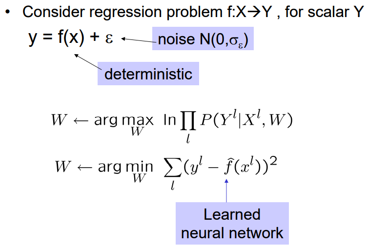Figure: MLE training for neural networks.

• Linear, logistic regression and multiclass logistic regression
• Conditional random field (CRF)
• Hidden Markov Model (HMM)

Maximum a Posteriori Estimation (MAP)

• Maximum a posteriori estimation (MAP) estimate parameter which has the maximum probability given data, instead of maximizing the probability of data given parameter (MLE).
  • MAP estimate chooses the point of maximal posterior probability or maximal probability density in the more common case of continuous \(\theta\).
  • As we can only observe \(p(x \mid \theta)\) (likelihood), we use Bayes’ Theroem to use \(p(\theta \mid x)\).

\[\theta_{MAP} = \arg\max_\theta p(\theta \mid x) = \arg\max_\theta log p(x \mid \theta) + \log p(\theta)\]

• MAP Bayesian inference has the advantage of leveraging information that is brought by the prior and connot be found in the training data.
  • This additional information helps to reduce the variance in the MAP point estimate compared to the MLE.
• MLE vs. MAP
  • Assume we train a logistic regression model,
    • MLE training: pick \(W\) to maximize \(P(Y \mid X, W)\)
    • MLE training: pick \(W\) to maximize \(P(W \mid X, Y)\)
  • If a prior information is given as part of the problem, then use MAP.
    • If not, we cannot use MAP and MLE is a reasonable approach.

MAP Usage

• Neural Network
  • MAP is closely related to the method of MLE, but employs an augmented optimization objective which incorporates a prior distribution over the quantity one want to estimate.
  • MAP estimation can therefore be seen as a regularization of MLE.

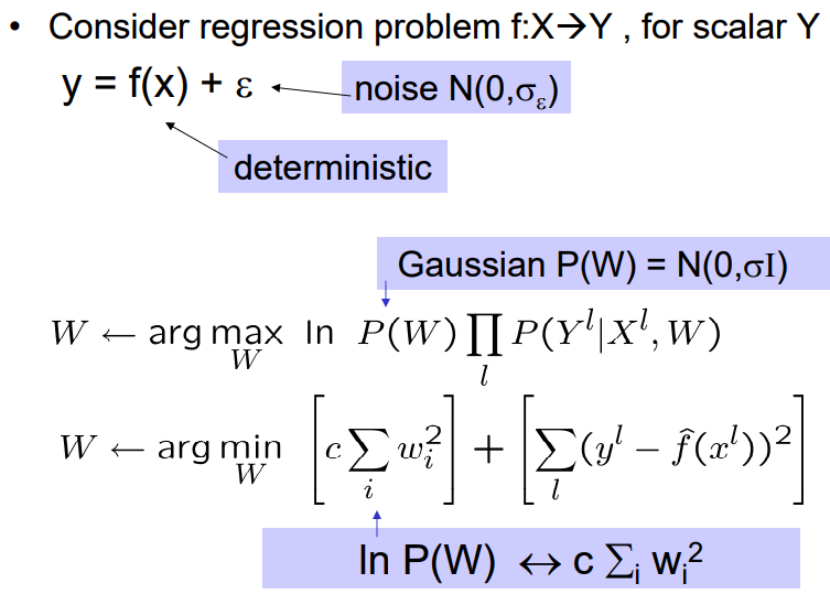Figure: MAP training for neural networks.

• Bayesian Neural Network
• Hidden Markov Model (HMM)

References

• Book: Deep Learning book [Link]
• Web: Standford CS109 Deep Learning Lecture material [Link]
• Web: CMU Neural Network Lecture material [Link]
• Wikipedia: Maximum a posteriori estimation [Link]