Approximate inference methods make it possible to learn realistic models from big data by trading off computation time for accuracy, when exact learning and inference are computationally intractable.
Approximate Inference
- In latent variable model, we might want to extract features \(E[h \mid v]\) describing the observed variables \(v\) (visible variable \(v\), a set of latent variables \(h\)).
- We often training our models using the principle of maximum likelihood.
- Because we often want to compute \(p(h \mid v)\) in order to implement a learning rule.
- This is inference problem in which we must predict the value of some variables given other variables, or predict the probability distribution over some variables given the value of other variables.
- Unfortunately, inference problems are intractable, because of computing \(p(h \mid v)\) or taking expectations with respect to it is difficult which are often necessary for tasks like maximum likelihood learning.
- Also, computing the marginal probability of a general graphical model is \(\# P\) hard which is a generalization of the complexity class \(NP\).
- So, exact inference requires an exponential amount of time in these models.
Inference as Optimization
- Decomposition of Log-Likelihood
- Approximate inference algorithms may be derived by approximating the underlying optimization problem.
- To construct the optimization problem, we would like to compute the log probability of the observed data, \(\log p(v; \theta)\).
- Sometimes, it is difficult to compute \(\log p(v;\theta)\) if it is costly to marginalize out \(h\).
- Instead, we can compute a lower bound \(\mathcal{L}(v,\theta,q)\) on \(\log p(v;\theta)\)
- This bound is called the evidence lower bound (ELBO) or the negative variational free energy.
- Where \(q\) is an arbitrary probability distribution over \(h\), the ELBO is defined to be:
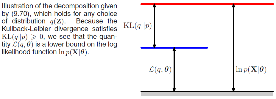
- Because the difference between \(\log p(v)\) and \(\mathcal{L}(v,\theta,q)\) is given by the KL divergence and because the KL divergence is always non-negative, we can see that \(\mathcal{L}\) always has at most the same value as the desired log probability.
- The two are equal if and only if \(q\) is the same distribution as \(p(h \mid v)\).
- \(\mathcal{L}\) can be considerably easier to compute for some distributions q.
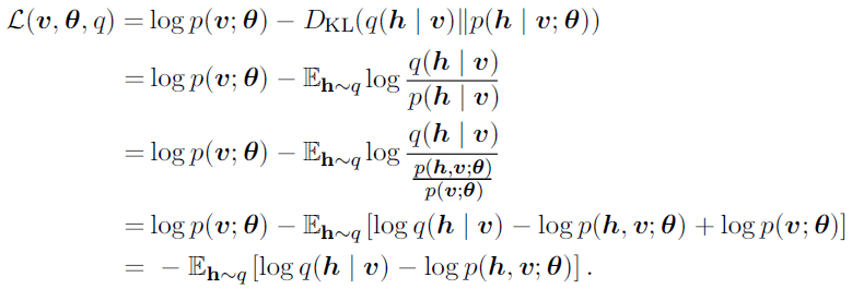
which leads the more canonical definition of the evidence lower bound,
- For an appropriate choice of \(q\), \(\mathcal{L}\) is tractable to compute.
- For any choice of \(q\), \(\mathcal{L}\) provides a lower bound on the likelihood.
- For \(q(h \mid v)\) that are better approximations of \(p(h \mid v)\), the lower bound \(\mathcal{L}\) will be tighter which is closer to \(\log p(v)\).
- When \(q(h \mid v) = p(h \mid v)\), the approximation is perfect, and \(\mathcal{L}(v,\theta,q)=\log p(v;\theta)\).
- We can think of inference as the procedure for finding the \(q\) that maximizes \(\mathcal{L}\).
- Exact inference maximizes \(\mathcal{L}\) perfectly by searching over a family of functions \(q\) that includes \(p(h \mid v)\).
- Below techniques are the way to derive different forms of approximate inference by using approximate optimization to find \(q\).
- No matter what choice of \(q\) we use, \(\mathcal{L}\) is as lower bound.
- We can get tighter or looser bounds that are cheaper or more expensive to compute depending on how we choose to approach this optimization problem.
Expectation Maximization
- Expectation Maximization (EM) is an algorithm for maximizing a lower bound \(\mathcal{L}\) which is popular training algorithm for models with latent variables.
- EM is not an approach to approximate inference, but rather an approach to learning with an approximate posterior.
- EM is widely used algorithm for MLE and MAP problem of probabilistic model with latent variable.
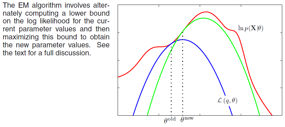
- The EM algorithm consists of alternating between two steps until convergence:
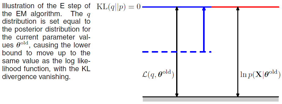
- E-step (Expectation step)
- We maximize \(\mathcal{L}\) with respect to \(q\).
- Let \(\theta^0\) denote that value of the parameters at the beginning of the step.
- Set \(q(h^i \mid v) = p(h^i \mid v^i; \theta^0)\) for all indices \(i\) of the training examples \(v^i\) we want to train on.
- By this we mean \(q\) is defined in terms of the current parameter value of \(\theta^0\); if we vary \(\theta\) then \(p(h \mid v;\theta)\) will change but \(q(h \mid v)\) will remain equal to \(p(h \mid v;\theta^0)\).
- E.g. In K-means clustering, E-step assigns the data points to the nearest centroid.
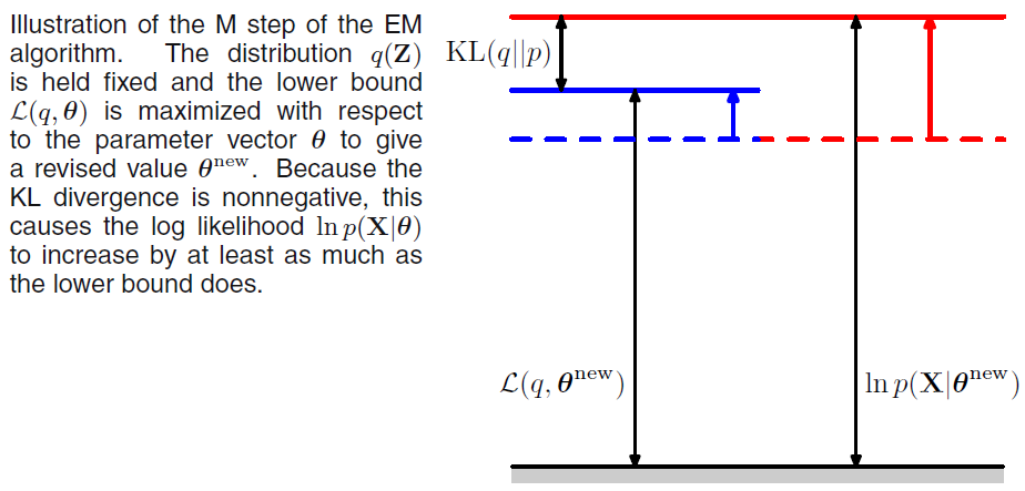
- M-step (Maximization step)
- We maximize \(\mathcal{L}\) with respect to \(\theta\).
- Completely or partially maximize with respect to \(\theta\) using your optimization algorithm of choice.
- E.g. In K-means clustering, M-step update the centroid positions given the assignments.
Variational Inference
- Variational inference is that we approximate the true distribution \(p(h \mid v)\) by seeking an approximate distribution \(q(h \mid v)\) that is as close to the true one as possible.
