Learn about Dynamic Programming which is a famous and important algorithm for solving problems.
Dynamic Programming
Dynamic programming is a method for solving a complex problem by following this steps:
- Break it down into a collection of simpler subproblems
- Solve each of subproblems just once and store their solutions
- When the same subproblem occurs, look up the previously computed solutions thereby saving computation time and space
- Memoization: The technique of storing solutions to subproblems instead of recomputing them.
Coin Changing Problem
Problem Statement
For a given set of denominations, find the minimum number of coins with which a given amount of money can be paid. Assume that you can use as many coins of a particular denomination as necessary.
Approach with Greedy Algorithm
- Process
- Using greedy algorithm, we can simply choose the largest denomination not exceeding the remaining amount of money to be paid.
- As long as the remaining amount is greater than zero, the process is repeated.
- Exception
- The algorithm may return a suboptimal result.
- For an amount of 6 and coins of values 1, 3, 4, we get 6 = 4+ 1+ 1, but the optimal solution here is 6 = 3 + 3.
Approach with Dynamic Programming
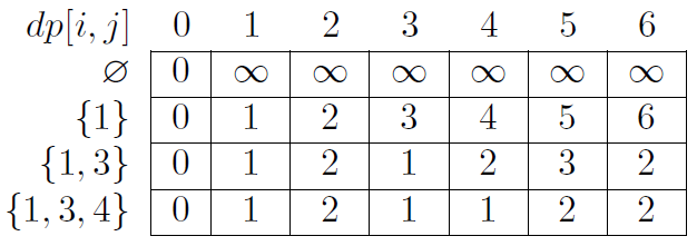
A dynamic algorithm finds solutions to this problem for all amounts not exceeding the given amount, and for increasing sets of denominations. For example, it would consider all the amounts from 0 to 6, and the following sets of denominations: \(\varnothing,\{1\},\{1,3\},\{1,3,4\}\). Let \(dp[i, j]\) be the minimum number of coins needed to pay the amount \(j\) if we use the set containing the \(i\) smallest denominations.
The number of coins needed must satisfy the following rules:
- no coins are needed to pay a zero amount: \(dp[i, 0] = 0\)
- if there are no denominations and the amount is positive, there is no solution: \(dp[0, j]=\infty\)
- if the amount to be paid is smaller than the highest denomination \(c_i\), this denomination can be discarded: \(dp[i,j] = dp[i-1,j]\)
- otherwise, either we use a coin of the highest denomination and a smaller amount to be paid remains, or we don’t use coins of the highest denomination: \(dp[i,j] = min(dp[i,j-c_i] + 1, dp[i-1,j])\)
The following table shows all the solutions to sub-problems considered for the example.
Implementation
Consider \(n\) denominations, \(0 \leq c_0 \leq c_1 \leq ... \leq c_{n-1}\). The algorithm processes the respective denominations and calculates the minimum number of coins needed to pay every amount from 0 to \(k\).
# In Python 3
# Time complexity and space complexity are O(nk)
import math
def dynamic_coin_changing(C, k):
    n = len(C)
    # Create two-dimensional array with all zeros
    dp = [[0]*(k+1) for _ in range(n+1)] # not same with [[0]*(k+1)]*(n+1)
    dp[0] = [0] + [math.inf] * k
    for i in range(1, n+1):
        for j in range(C[i-1]):
            dp[i][j] = dp[i-1][j]
        for j in range(C[i-1], k+1):
            dp[i][j] = min(dp[i][j-C[i-1]] + 1, dp[i-1][j])
     return dp[n]
- Space optimized version: during the calculation of \(dp\), we only use the previous row, so we don’t need to remember all of the rows.
# In Python 3
import math
def dynamic_coin_changing(C, k):
    n = len(C)
    dp = [0] + [math.inf] * k
    for i in range(1, n+1):
        for j in range(C[i-1], k+1):
            dp[j] = min(dp[j-C[i-1]] + 1, dp[j])
    return dp
Frog Problem
Problem Statement
A small frog wants to get from posiiton 0 to \(k\) (\(1 \leq k \leq 10000\)). The frog can jump over any one of \(n\) fixed distance \(s_0, s_1, ..., s_{n-1} (1\leq s_i \leq k)\). The goal is to count the number of different ways in which the frog can jump to position \(k\). To avoid overflow, it is sufficient to return the result modulo \(q\), where \(q\) is a given number.
Approach with Dynamic Programming
Create an array \(dp\) consisting of \(k\) elements, such that \(dp[j]\) will be the number of ways in which the frog can jump to position \(j\). We update consecutive cells of array \(dp\). There is exactly one way for the frog to jump to position 0, so \(dp[0]=1\).
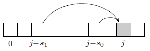
The number of ways in which the frog can jump to position \(j\) with a final jump of \(s_i\) is \(dp[j-s_i]\). Thus, the number of ways in which the frog can get to position \(j\) is increased by the number of ways of getting to position \(j-s_i\), for every jump \(s_i\). More precisely, \(dp[j]\) is increased by the value of \(dp[j-s_i]\) modulo \(q\).
Implementation
- Time complexity: \(O(nk)\)
- Space complexity: \(O(k)\)
def frog(S, k, q):
    n = len(S)
    dp = [1] + [0]*k #[1] for the case of jumping to position 0
    for j in range(1, k+1):
        for i in range(n):
            if S[i] <= j:
                dp[j] = (dp[j] + dp[j - S[i]] % q
    return dp[k]