Learn about tree, tree traversal, binary heap, trie and their running time.
Tree
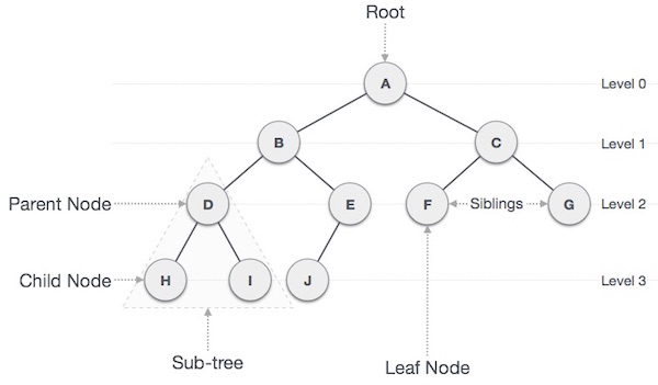
- Tree is a data structure composed of nodes.
- Each tree has a root node.
- The root node has zero or more child nodes.
- Each child node has zero or more child nodes, and so on.
- Features of tree
- Tree cannot contain cycles.
- The nodes may or may not be in a particular order.
- They may or may not have links back to their parent nodes.
Trees vs. Binary Trees
- Binary tree is a tree in which each node has up to two children.
- Other than that, it will be \(n\)-ary tree.
- A node is called a leaf node if it has no children.
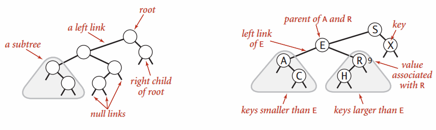
Binary Tree vs. Binary Search Tree
- Binary search tree is a binary tree in which every node fits a specific ordering property:
- For each node \(n\), \(\text{all left descendents} <= n < \text{all right descendents}\)
- In some definitions, the tree cannot have duplicate values.
- In others, the duplicate values will be on the right or can be on either side.
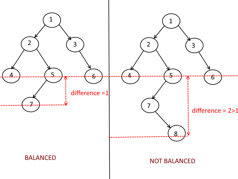
Balanced vs. Unbalanced
- In order to guarantee that \(H = \log N\) (\(H\):height, \(N\): number of nodes), we can force the tree to be height-balanced.
- Relation between \(H\) and \(N\) in a tree can vary from \(H=N\) (degenerate tree) to \(H=\log N\).
- Two common types of balanced trees are red-black trees and AVL trees
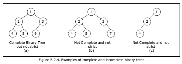
Complete Binary Trees
- Complete binary tree is a binary tree in which every level of the tree is fully filled, except for perhaps the last level.
Full Binary Trees
- Full binary tree is a binary tree in which every node has either zero or two children, no nodes have only one child.
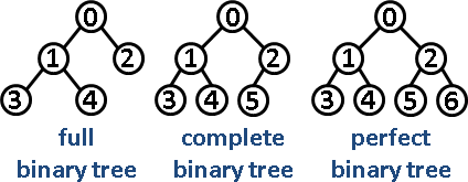
Perfect Binary Trees
- Perfect binary tree is one that is both full and complete.
- A perfect tree must have exactly \(2^k-1\) nodes where \(k\) is the number of levels.
Binary Tree Traversal
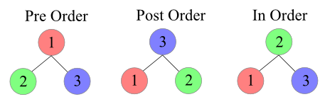
Pre-Order Traversal
- In a pre-order traversal, the root of tree is visited first and then the subtrees rooted at its children are traversed recursively.
- Time complexity: \(O(n)\), where \(n\) is the number of positions in the tree.
Algorithm preorder(T, p):
    perform the "visit" action for position p
    for each child c in T.children(p) do
        preorder(T,c) # recursively traverse the subtree rooted at c
Post-Order Traversal
- In a post-order traversal, it recursively traverses the subtrees rooted at the children of the root first, and then visits the root.
- Time complexity: \(O(n)\), where \(n\) is the number of positions in the tree.
Algorithm postorder(T, p):
    for each child c in T.children(p) do
        postorder(T,c) # recursively traverse the subtree rooted at c
    perform the "visit" action for position p
In-Order Traversal
- In a in-order traversal, for every position p, the inorder traversal visits p after all the positions in the left subtree of p and before all the positions in the right subtree of p.
- Time complexity: \(O(n)\), where \(n\) is the number of positions in the tree.
Algorithm inorder(p):
    if p has a left child lc then
        inorder(lc) # recursively traverse the left subtree of p
    perform the "visit" action for position p
    if p has a right child rc then
        inorder(rc) # recursively traverse the right subtree of p
Binary Heaps (Min-Heaps and Max-Heaps)
- Min-heap is a complete binary tree where each node is smaller than its children.
- The root is the minimum element in the tree.
- Max-heap is essentially equivalent but the elements are in descending order rather than ascending order.
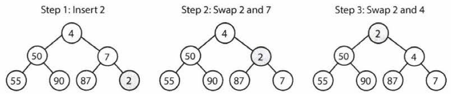
Insert
- Insert element at the rightmost spot, then we fix the tree by swapping the new element with its parent, until we find an appropriate spot for the element.
- Takes \(O(\log n)\) time, where \(n\) is the number of nodes in the heap.
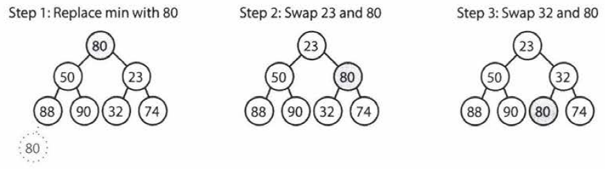
Extract Minimum Element
- First, we remove the minimum element and swap it with the last element in the heap.
- Then, we bubble down this element, swapping it with one of its children until the min-heap property is restored.
- Takes \(O(\log n)\) time, where \(n\) is the number of nodes in the heap.
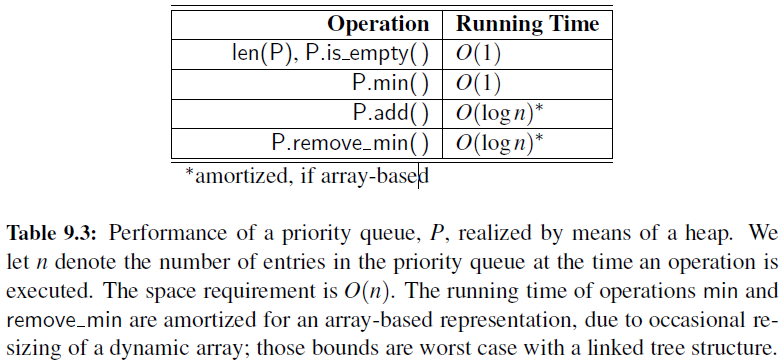
Analysis of a Heap-Based Priority Queue
Python’s heapq Module
- Python’s standard distribution includes a heapq module that provides support for min-heap priority queues.
- Functions: heappush(L,e), heappop(L), heappushpop(L,e), heapreplace(L,e), heapify(L), nlargest(k,iterable), nsmallest(k,iterable)
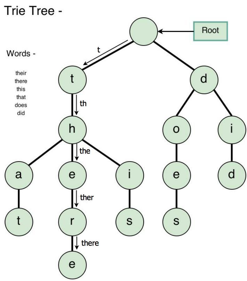
Tries (Prefix Trees)
- Trie is a variant of an n-ary tree in which characters are stored at each node.
- Each path down the tree may represent a word.
- The * nodes (null nodes) are often used to indicate complete words.
- A node in a trie could have anywhere from 1 through \(\text{alphabet_size}+1\) children (or, 0 if a boolean flag is used instead of a * node).
- A trie can check if a string is a valid prefix in \(O(k)\) time, where \(k\) is the length of the string.