Autoencoder is an artificial neural network used for unsupervised learning of efficient codings. The aim of an autoencoder is to learn a representation (encoding) for a set of data, typically for the purpose of dimensionality reduction. Recently, the autoencoder concept has become more widely used for learning generative models of data.
Autoencoder, 1989
- For the intuitive understanding, autoencoder compresses (learns) the input and then reconstruct (generates) of it.
- It is unsupervised learning model which does not need label.
\[\text{Input'} = \text{Decoder(Encoder(Input))}\]
Structure
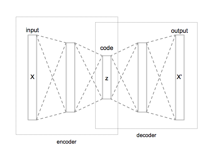
- Basic form of an autoencoder is a feedforward neural network which has an input layer, an output layer and one or more hidden layers.
- Output layer has the same number of nodes as the input layer for reconstructing its own inputs.
- An autoencoder consists of two parts, the encoder \(\phi\) and the decoder \(\psi\)
- They will be chosen by minimizing the distance between \(X\) and \(X'\).
\[\phi:\mathcal{X} \rightarrow \mathcal{F} \\
\psi:\mathcal{F} \rightarrow \mathcal{X} \\
\phi,\psi = \underset{\phi,\psi}{\operatorname{arg\,min}}\, \|X-(\psi \circ \phi) X\|^2\]
- The encoder stage of an autoencoder take the input \(\mathbf{x} \in \mathbb{R}^d = \mathcal{X}\) and maps it to \(\mathbf{z} \in \mathbb{R}^p = \mathcal{F}\).
- The \(z\) is referred to as code, latent representation.
- \(W\) is a weight, \(b\) is a bias vector, \(\sigma\) is activation function for non-linearity.
- The decoder stage of the autoencoder maps \(z\) to the reconstruction \(x'\) of the same shape as \(x\).
\[\mathbf{z} = \sigma(\mathbf{Wx}+\mathbf{b})
\mathbf{x'} = \sigma'(\mathbf{W'z}+\mathbf{b'})\]
- Loss function: Autoencoder is trained to minimise reconstruction error (squared error) where \(x\) is usually averaged over some input training set.
\[\mathcal{L}(\mathbf{x},\mathbf{x'})=\|\mathbf{x}-\mathbf{x'}\|^2=\|\mathbf{x}-\sigma'(\mathbf{W'}(\sigma(\mathbf{Wx}+\mathbf{b}))+\mathbf{b'})\|^2\]
Autoencoder for PCA
The first paper suggested autoencoder (Baldi, P. and Hornik, K. 1989) proposed the implementation of PCA using backpropagation of neural network
PCA
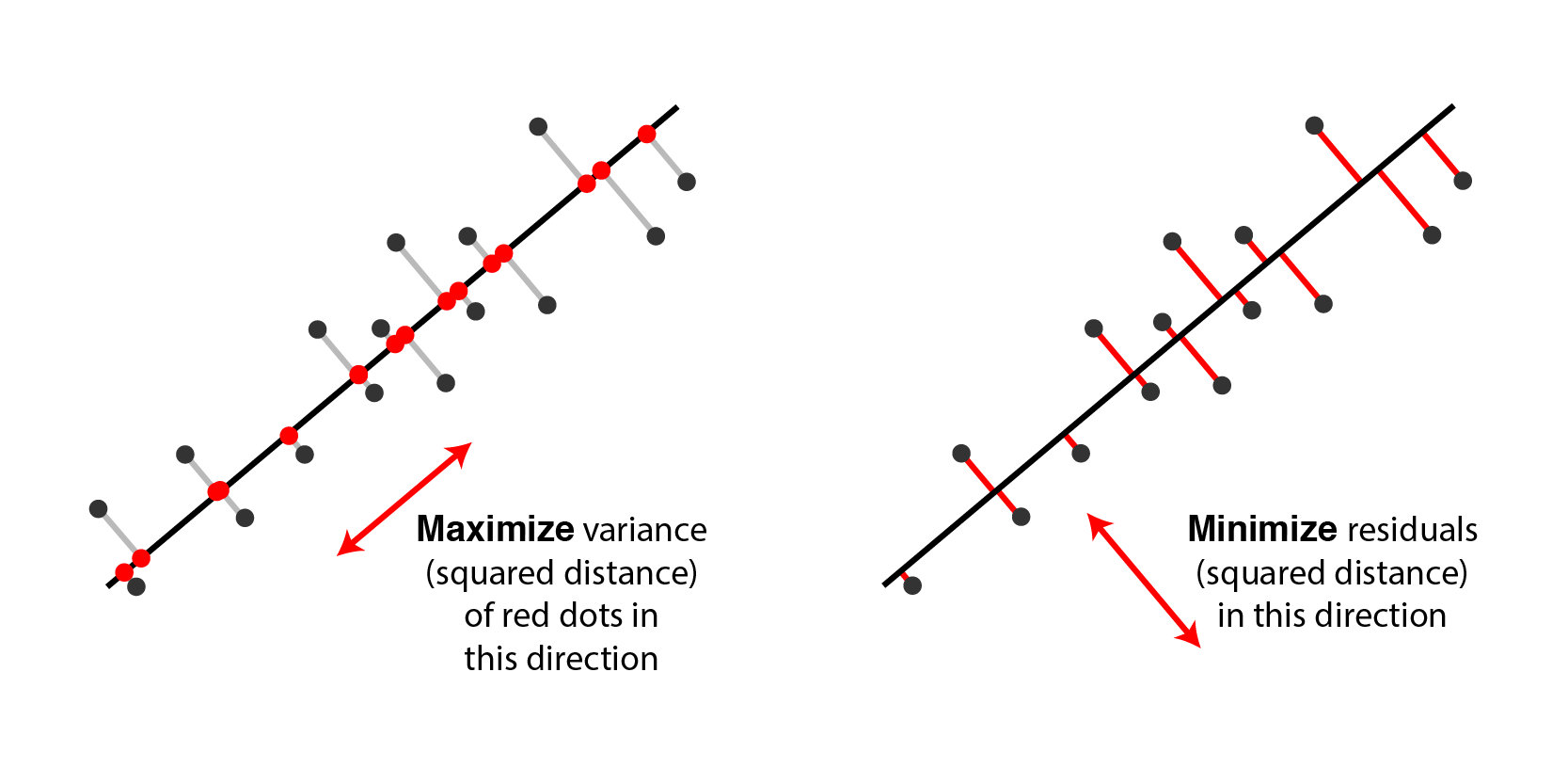
- PCA takes N-dimentional data and finds the M orthogonal directions in which the data have the most variance.
- These M principal directions form a lower-dimensional subspace.
- We can represent an N-dimensional datapoint by its projections onto the M principal directions.
- This loses all information about where the datapoint is located in the remaining orthogonal directions.
- We reconstruct by using the mean value (over all the data) on the N-M directions that are not represented.
- The reconstruction error (squared distance) is the sum over all these unrepresented directions of the squared differences of the datapoint from the mean.
PCA Using Autoencoder
- If the hidden and output layers are linear, it will learn hidden units that are a linear function of the data and minimize the squared reconstruction error which is exactly what PCA does.
- Autoencoder will be trained to minimise the reconstruction error which tries to make input \(x\) and output \(x'\) the same.
- The code \(z\) with \(M\) hidden unit will be compressed representation of input \(N\)
- It is usually inefficient than PCA, which can be improved with big data set.
- The M hidden units will span the same space as the first M components found by PCA.
- Their weight vectors may not be orthogonal.
- They will tend to have equal variances.
- With non-linear layers before and after the code, it should be possible to efficiently represent data that lies on or near a non-linear manifold.
- The encoder converts coordinates in the input space to coordinates on the manifold.
- The decoder does the inverse mapping
Deep Autoencoder, 2006
Before we talk about deep autoencoder, we have to know about restricted boltzmann machine and deep belief networks.
Restricted Boltzmann Machine (RBM)
- Restricted Boltzmann Machine (RBM) is a generative stochastic artificial neural network that can learn a probability distribution over its set of inputs.
- RBM is a variant of Boltzmann machines with the restriction that their neurons much form a bipartite graph and there are no connections between nodes within a group.
- This restriction allows for more efficient training algorithm, in particular the gradient-based contrastive divergence algorithm.
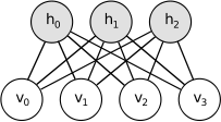
- The standard type of RBM has binary-valued (Boolean/Bernoulli) hidden and visible units, and consists of a matrix of weights \(W\), bias term \(a_i\) for the visible units and \(b_j\) for the hidden units.
- This model contains joint probability of \(v\) and \(h\) which can be described with energy function form,
\[p(v,h) = \frac{e^{-E(v,h)}}{Z} \\
\mbox{ where } E(v,h) := -\sum_i a_i v_i - \sum_j b_j h_j - \sum_i \sum_j v_i w_{ij} h_j \\
\mbox{ and } Z = \sum_{v,h} e^{-E(x,h)}\]
- RBM will be trained in a way that best describes the given data, that is, the parameter that maximizes \(p(v)\) is learned.
- This usually described with log likelihood as,
\[\theta = \arg\max_\theta \log \mathcal L (v) = \arg\max_\theta \sum_{v \in V} \log P(v).\]
- RBM reduced training and inference time compared to Boltzmann machine
- And it can be used in both supervised and unsupervised learning such as dimensionality reduction, classification, collaborative filtering, feature learning, topic modeling.
Deep Belief Network (DBN)
- Deep Belief Network (DBN) is a generative graphical model, composed of multiple layers of hidden units with connections between the layers but not between units within each layer.
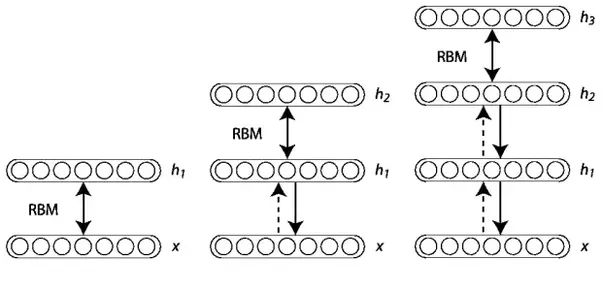
- It can consist of stacking RBM from the bottom and update parameters
- When trained on a set of examples without supervision, a DBN can learn to probabilistically reconstruct its inputs.
- The layers then act as feature detectors.
- After this learning step, a DBN can be further trained with supervision to perform classification.
- When \(h^k\) is the hidden variable of k-th layers, DBN probabilistic model can be described as,
\[P(x, h^1, \ldots, h^\ell) = \bigg( \prod_{k=1}^{\ell-2} P(h^k|h^{k-1}) \bigg) P(h^{\ell-1},h^{\ell})\]
- Pre-training with DBN and fine-tuning with backpropagation improved performance on MNIST dataset classification.
- Unsupervised pre-training with DBN also showed better performance than before.
- However, these days, when there is enough big data set, random initialization gives better performance than pre-training with DBN.
Deep Autoencoder (Stacked Autoencoder)
- Deep autoencoder is a nice way to do non-linear dimensionality reduction
- Provide flexible mappings both ways
- The learning time is linear (or better) in the number of training cases
- The final encoding model is fairly compact and fast
- It also showed good reconstruction performance
- However, it turned out to be very difficult to optimize deep autoencoders using backpropagation
- With small initial weights the backpropagated gradient dies
- Now, we have a better ways to optimize them
- Use unsupervised layer-by-layer pre-training.
- Or just initialize the weights carefully as in Echo-State Nets.
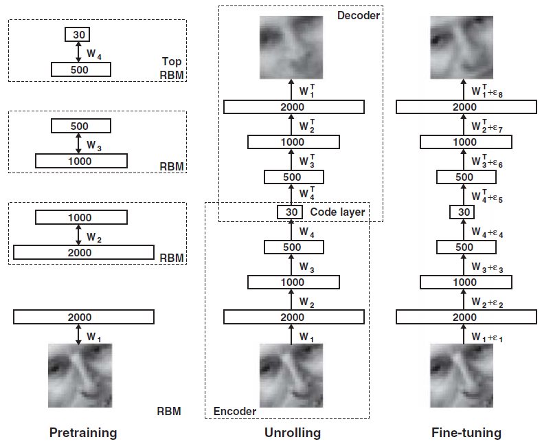
- Training process
- Pretraining: Learn a stack of RBMs, each having only one layer of feature detector and the learned feature activations of one RBM are used as the “data” for training next RBM in the stack.
- Unrolling: Create a deep autoencoder, use transpose of encoder weight for decoder weight.
- Fine-tuning: Fine-tune the model using backpropagation of error derivatives
Denoising Autoencoder, 2008
- Denoising autoencoder take a partially corrupted input while training to recover the original undistorted input.
- A good representation is one that can be obtained robustly from a corrupted input and that will be useful for recovering the corresponding clean input.
- This definition contains the following implicit assumptions
- The higher level representations are relatively stable and robust to the corruption of the input.
- It is necessary to extract features that are useful for representation of the input distribution.
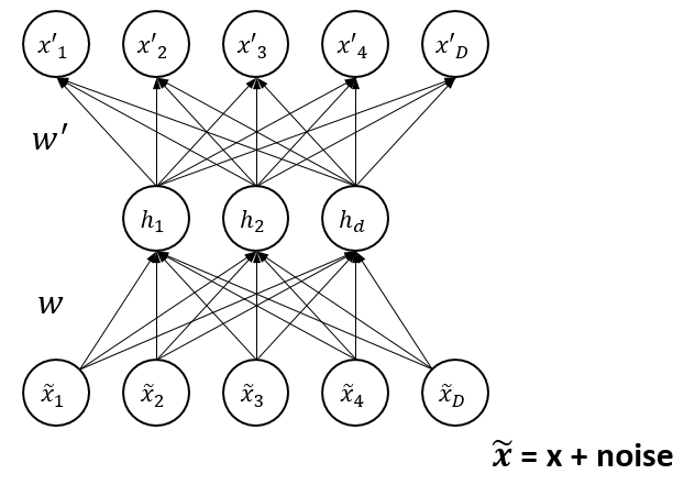
- To train an autoencoder to denoise data, it is necessary to perform preliminary stochastic mapping \(\mathbf{x}\rightarrow\mathbf{\tilde{x}}\) in order to corrupt the data
- And use \(\mathbf{\tilde{x}}\) as input for a normal autoencoder
- The loss should be still computed for the initial input \(\mathcal{L}(\mathbf{x},\mathbf{\tilde{x}'})\) instead of \(\mathcal{L}(\mathbf{\tilde{x}},\mathbf{\tilde{x}'})\).
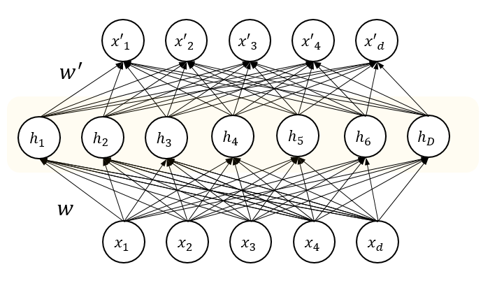
Sparse Autoencoder, 2008
- By imposing sparsity on the hidden units during training (having a larger number of hidden units than inputs), an autoencoder can learn useful structures in the input data.
- This allows sparse representations of inputs which is useful in pretraining for classification tasks.
- Sparsity may be achieved by additional terms in the loss function during training or by manually zeroing all but the few strongest hidden unit activations.
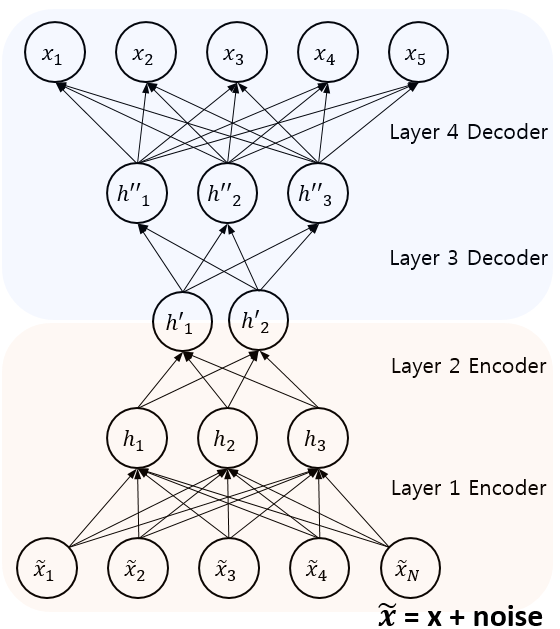
Stacked Denoising Autoencoder, 2010
- A stacked denoising autoencoder is a stacked of denoising autoencoder by feeding the latent representation (output code) of the denoising autoencoder as input to the next layer.
- A key function of SDAs is unsupervised pre-training, layer by layer, as input is fed through.
- Once each layer is pre-trained to conduct feature selection and extraction on the input from the preceding layer, a second stage of supervised fine-tuning can follow.
Variational Autoencoder, 2013
- Variational autoencoder is a generative model for complex data and large dataset proposed in 2013 by Kingma et al. and Rezende et al..
- It can generate images of fictional celebrity faces and high-resolution digital artwork.
- It achieved state-of-the-art machine learning results in image generation and reinforcement learning.

Encoder
- The encoder is a neural network and its input is a datapoint \(x\), output is a hidden representation \(z\), and it has weights and biases \(\theta\).
- The representation space \(z\) is less than the input space and it is referred to as a bottleneck because the encoder must learn an efficient compression of the data into this lower-dimensional space.
- The lower-dimensional space is stochastic where the encoder outputs parameters to \(q_{\theta}(z \mid x)\) which is a Gaussian probability density.
- We can sample from this distribution to get noisy values of the representations \(z\).
Decoder
- The decoder is another neural network and its input is the representation \(z\), output is the parameters to the probability distribution of the data, and it has weights and biases \(\phi\).
- The decoder is denoted by \(p_{\phi}(x \mid z)\).
- The decoder gets as input the latent representation of a digit \(z\) and decodes it into real-valued numbers between 0 and 1 (when it is Bernoulli parameters).
- Information is lost because it goes from a smaller to a larger dimensionality and this can be measured by reconstruction log-likelihood \(\log p_{\phi}(x \mid z)\).
- This measure tells us how effectively the decoder has learned to reconstruct an input image \(x\) given its latent representation \(z\).
Loss Function
- THe loss function of the variational autoencoder is the negative log-likelihood with a regularizer.
- Because there are no global representations that are shared by all datapoints, we can decompose the loss function into only terms that depend on a single datapoint \(l_i\).
- The total loss is then \(\sum_{i=1}^N l_i\) for \(N\) total data points.
- The loss function \(l_i\) for datapoint \(x_i\) is:
\[l_i(\theta, \phi) = -E_{z \sim q_{\theta}(z \mid x_i)}[\log p_{\phi}(x_i \mid z)] + KL(q_{\theta}(z \mid x_i) \parallel p(z))\]
- The first term is the reconstruction loss, or expected negative log-likelihood of the \(i\)-th datapoint.
- This term encourages the decoder to learn to reconstruct the data.
- If the decoder’s output does not reconstruct the data well, it will incur a large cost in this loss function.
- The second term is a regularizer that is the Kullback-Leibler divergence between the encoder’s distribution \(q_{\theta}(z \mid x)\) and p(z).
- The divergence measures how much information is lost when using \(q\) to represent \(p\) and how close \(q\) is to \(p\).
- We train the variational autoencoder using gradient descent to optimize the loss with respect to the parameters of the encoder and decoder.
- For stochastic gradient descent with step size \(\rho\), the encoder parameters are updated using \(\theta \leftarrow \theta - \rho \frac{\partial l}{\partial \theta}\) and the decoder is updated similarly.
References
- Wikipedia: Autoencoder [Link]
- Youtube: From PCA to autoencoders [Neural Networks for Machine Learning] [Link]
- Paper: Neural Networks and Principal Component Analysis: Learning from Examples Without Local Minima [Link]
- Paper: Reduction the Dimensionality of Data with Neural Network, Science [Link]
- Blog: Tutorial - What is a variational autoencoder? [Link]